Sections in this Chapter:
- Convexity
- Gradient descent
- Root-finding
- General purpose minimization tools
- Linear programming
- Miscellaneous
We are talking about mathematical optimization in this chapter. Mathematical optimization is the selection of a best element from some set of available alternatives. Why we talk about optimization in this book on data science? Data science is used to help make better decisions, and so is optimization. Operations Research, with optimization at its core, is a discipline that deals with the application of advanced analytical methods to make better decisions1. I always feel Data Science and Operations Research are greatly overlapped. The training of a variety of (supervised) machine learning models is to minimize the loss functions, which is essentially an optimization problem. In optimization, the loss functions are usually referred as objective functions.
Mathematical optimization is a very broad field and we ignore the theories in the book and only touch some of the simplest applications. Actually, in Chapter 4 we have seen one of its important applications in linear regression.
Convexity
The importance of convexity cannot be overestimated. A convex optimization problem2 has the following form
$$
\begin{equation}
\begin{split}
&\max_{\boldsymbol{x}} {f_0(\boldsymbol{x})}\\
&subject\quad to\quad f_i(\boldsymbol{x})\leq{\boldsymbol{b}_i};i=1,…,m,
\end{split}
\label{eq:convex}
\end{equation}
$$
where the vector $\boldsymbol{x}\in\mathbf{R}^n$ represents the decision variable; $f_i;i=1,…,m$ are are convex functions ($\mathbf{R}^n\rightarrow\mathbf{R}$). A function $f_i$ is convex if
$$
\begin{equation}\label{eq:convex2}
f_i(\alpha\boldsymbol{x}+(1-\alpha)\boldsymbol{y})\leq {\alpha f_i(\boldsymbol{x})+ (1-\alpha) f_i(\boldsymbol{y})},
\end{equation}
$$
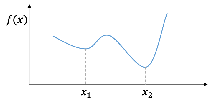
for all $\boldsymbol{x}$, $\boldsymbol{y}$ $\in\mathbf{R}^n$, and all $\alpha$ $\in\mathbf{R}$ with $0\leq\alpha\leq1$. \eqref{eq:convex} implies that a convex optimization problem requires both the objective function and the set of feasible solutions are convex. Why do we care the convexity? Because convex optimization problem has a very nice property – a local minimum (which is minimal among a neighboring set of candidate solutions) is also a global minimum (which is the minimal solution among all feasible solutions). Thus, if we can find a local minimum we get the global minimum for convex optimization problems.
Many methods/tools we will introduce in the following sections won’t throw an error if you feed them a non-convex objective function; but the solution returned by these numerical optimization methods are not necessary to be a global optimum. For example, the algorithm may get trapped in a local optimum.
Gradient descent
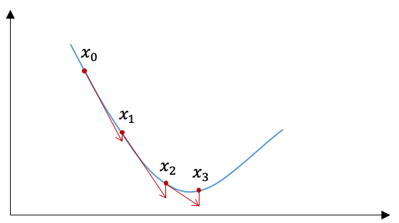
What is the most commonly used optimization algorithm in machine learning? Probably the answer is gradient descent (and its variants). The gradient descent is also an iterative method, and in step $i$ the update of $\boldsymbol{x}$ follows
$$
\begin{equation}
\begin{split}
\boldsymbol{x}^{(k+1)}=\boldsymbol{x}^{(k)}-\gamma\nabla f(\boldsymbol{x}^{(k)}),
\end{split}
\label{eq:5_gradient_descent}
\end{equation}
$$
where $f$ is the objective function and $\gamma$ is called the step size or learning rate. Start from an initial value $\boldsymbol{x}_0$ and follow \eqref{eq:5_gradient_descent}, we will have a monotonic sequence $f(\boldsymbol{x}^{(0)})$, $f(\boldsymbol{x}^{(1)})$, …, $f(\boldsymbol{x}^{(n)})$ in the sense that $f(\boldsymbol{x}^{(k)})>=f(\boldsymbol{x}^{(k+1)})$. When the problem is convex, $f(\boldsymbol{x}^{(i)})$ converges to the global minimum.
Many machine learning models can be solved by the gradient descent algorithm, for example, the linear regression (with or without penalty) introduced in Chapter 5. Let’s see how to use the vanilla (standard) gradient descent method in linear regression we introduced in Chapter 5.
According to the gradient derived in Chapter 5, the update for the parameters become:
$$
\begin{equation}
\begin{split}
\boldsymbol{\hat{\beta}}^{(k+1)}=\boldsymbol{\hat{\beta}}^{(k)}+2\gamma \boldsymbol{X}’(\boldsymbol{y}-\boldsymbol{X}\boldsymbol{\hat{\beta}}^{(k)}).
\end{split}
\end{equation}
$$
chapter6/linear_regression_gradient_descent.R
 1 library(R6)
 2 LR_GD = R6Class(
 3   "LR_GD",
 4   public = list(
 5     coef = NULL,
 6     learning_rate = NULL,
 7     x = NULL,
 8     y = NULL,
 9     seed = NULL,
10     initialize = function(x, y, learning_rate = 0.001, seed = 42) {
11       # we add 1s to x
12       self$x = cbind(1, x)
13       self$y = y
14       self$seed = seed
15       set.seed(self$seed)
16       # we use a fixed learning rate here, but it can also be adaptive
17       self$learning_rate = learning_rate
18       # let's initialize the coef
19       self$coef = runif(ncol(self$x))
20     },
21     fit = function(max_iteration = 1000) {
22       for (i in 1:max_iteration) {
23         self$update()
24       }
25     },
26     gradient = function() {
27       y_hat = self$predict(self$x)
28       # we normalize the gradient by the sample size
29       - 2 * (t(self$x) %*% (self$y - y_hat)) / nrow(self$x)
30     },
31     update = function() {
32       self$coef = self$coef - self$learning_rate * self$gradient()
33     },
34     predict = function(new_x) {
35       new_x %*% self$coef
36     }
37   )
38 )
Accordingly, we have the Python implementation as follows.
chapter6/linear_regression_gradient_descent.py
 1 class LR_GD:
 2     """
 3     linear regression with vanilla gradient descent
 4     """
 5
 6     def __init__(self, x, y, learning_rate=0.005, seed=42):
 7         # we put 1s in the first column of x
 8         self.x = np.hstack((np.ones((x.shape[0], 1)), x))
 9         self.y = y[:, None]
10         self.seed = seed
11         np.random.seed(self.seed)
12         self.coef = np.random.uniform(size=(self.x.shape[1], 1))
13         self.learning_rate = learning_rate
14
15     def predict(self, new_x):
16         # let's use @ for matrix multiplication
17         return new_x @ self.coef
18
19     def gradient(self):
20         y_hat = self.predict(self.x)
21         return -2.0*self.x.T @ (self.y-y_hat)/self.x.shape[0]
22
23     def update(self):
24         self.coef -= self.learning_rate*self.gradient()
25
26     def fit(self, max_iteration=1000):
27         for _ in range(max_iteration):
28             self.update()
Let’s use simulated dataset to test our algorithm.
 1 > source('gradient_descent.R')
 2 > n = 1000
 3 > set.seed(42)
 4 > x = cbind(rnorm(n), runif(n))
 5 > b = 6 # intercept
 6 > coef = c(2, 3)
 7 > err = runif(n, 0, 0.2)
 8 > y = x %*% coef + b + err
 9 > lr_gd = LR_GD$new(x = x, y = y, learning_rate = 0.05)
10 > lr_gd$fit(1000)
11 > lr_gd$coef
12          [,1]
13 [1,] 6.106233
14 [2,] 2.001042
15 [3,] 2.992593 1 >>> from gradient_descent import LR_GD
2 >>> import numpy as np
3 >>> n = 1000
4 >>> np.random.seed(42)
5 >>> x = np.column_stack((np.random.normal(size=n), np.random.uniform(size=n)))
6 >>> b = 6 # intercept
7 >>> coef = np.array([2, 3])
8 >>> err = np.random.uniform(size=n, low=0, high=0.2)
9 >>> y = x @ coef + b + err
10 >>> lr_gd = LR_GD(x=x, y=y, learning_rate=0.05)
11 >>> lr_gd.fit(1000)
12 >>> print(lr_gd.coef)
13 [[6.09887817]
14 [2.00028507]
15 [2.99996673]]The results show that our implementation of gradient descent update works well on the simulated dataset for linear regression.
However, when the loss function is non-differentiable, the vanilla gradient descent algorithm \eqref{eq:5_gradient_descent} cannot be used. In Chapter 5, we added the $L^2$ norm (also referred as Euclidean norm3) of $\boldsymbol{\beta}$ to the loss function to get the ridge regression. What if we change the $L^2$ norm to $L^1$ norm in the loss function?
$$
\begin{equation}\label{eq:5_lasso}
\min_{\boldsymbol{\hat\beta}} \quad \boldsymbol{e}’\boldsymbol{e} + \lambda \sum_{i=1}^p {|\boldsymbol{\beta}_i|},
\end{equation}
$$
where $\lambda>0$.
Solving the optimization problem specified in \eqref{eq:5_lasso}, we will get the Lasso solution of linear regression. Lasso is not a specific type of machine learning model. Actually, Lasso refers to least absolute shrinkage and selection operator. It is a method that performs both variable selection and regularization. What does variable selection mean? When we build up a machine learning model, we may collect as many data points (also called features, or independent variables) as possible. However, if only a subset of these data points are relevant for the task, we may need to select the subset explicitly for some reasons. First, it’s possible to reduce the cost (time or money) to collect/process these irrelevant variables. Second, adding irrelevant variables into the some machine learning models may impact the model performance. But why? Let’s take linear regression as an example. Including an irrelevant variable into a linear regression model is usually referred as model misspecification (Of course, omitting a relevant variable also results in a misspecified model). In theory, the estimator of coefficients is still unbiased ($\hat{\theta}$ is an unbiased estimator of $\theta$ if $E(\hat{\theta})=\theta$) when an irrelevant variable is included. But in practice, when the irrelevant variable has non-zero sample correlation coefficient with these relevant variables or the response variable $\boldsymbol{y}$, the estimate of coefficient may get changed. In addition, the estimator of coefficients are inefficient4. Thus, it’s better to select the relevant variables for a linear regression.
The Lasso solution is very important in machine learning because of its sparsity, which results in the automated variable selection. As for why the Lasso solution is sparse, the theoretical explanation could be found from the reference book5. Let’s focus on how to solve it. Apparently, gradient descent algorithm cannot be applied directly to solve \eqref{eq:5_lasso} although it is still a convex optimization problem since the regularized loss function is non-differentiable because of $||$.
Proximal gradient One of the algorithms that can be used to solve \eqref{eq:5_lasso} is called proximal gradient descent6. Let’s skip the theory of proximal methods and the tedious linear algebra, and jump to the solution directly. By proximal gradient descent, the update is given as follows in each iteration
$$
\begin{equation}
\begin{split}
\boldsymbol{\beta}^{(k+1)} &= S_{\lambda \gamma}(\boldsymbol{\beta}^{(i)}-2\gamma \nabla{(\boldsymbol{e}’\boldsymbol{e} )})) \\
&= S_{\lambda \gamma}(\boldsymbol{\beta}^{(i)}+2\gamma \boldsymbol{X}’(\boldsymbol{y}-\boldsymbol{X}\boldsymbol{\beta}^{(i)})) ,
\end{split}
\label{eq:5_lasso_1}
\end{equation}
$$
where $S_{\theta}(\cdot)$ is called soft-thresholding operator given by
$$
\begin{equation}\label{eq:sto}
[S_{\theta}(\boldsymbol{z})]_i =\left\{\begin{array}{ll} \boldsymbol{z}\sb{i} – \theta & \boldsymbol{z}\sb{i}>\theta;\\
0 & |\boldsymbol{z}\sb{i}|\leq\theta; \\
\boldsymbol{z}\sb{i} + \theta & \boldsymbol{z}\sb{i}<-\theta.
\end{array} \right.
\end{equation}
$$
Now we are ready to implement the Lasso solution of linear regression via \eqref{eq:sto}. Similar to ridge regression, we don’t want to put penalty on the intercept, and a natural estimate of the intercept is the mean of response, i.e., $\bar{\boldsymbol{y}}$. The learning rate $\gamma$ in each update could be fixed or adapted (change over iterations). In the implementation below, we use the largest eigenvalue of $\boldsymbol{X}’\boldsymbol{X}$ as the fixed learning rate.
chapter5/lasso.R
 1 library(R6)
 2
 3 # soft-thresholding operator
 4 sto = function(z, theta){
 5   sign(z)*pmax(abs(z)-rep(theta,length(z)), 0.0)
 6 }
 7
 8 Lasso = R6Class(
 9   "LassoLinearRegression",
10   public = list(
11     intercept = 0,
12     beta = NULL,
13     lambda = NULL,
14     mu = NULL,
15     sd = NULL,
16     initialize = function(lambda) {
17       self$lambda = lambda
18     },
19     scale = function(x) {
20       self$mu = apply(x, 2, mean)
21       self$sd = apply(x, 2, function(e) {
22         sqrt((length(e)-1) / length(e))*sd(e)
23       })
24     },
25     transform = function(x) t((t(x) - self$mu) / self$sd),
26     fit = function(x, y, max_iter=100) {
27       if (!is.matrix(x)) x = data.matrix(x)
28       self$scale(x)
29       x_transformed = self$transform(x)
30       self$intercept = mean(y)
31       y_centered = y - self$intercept
32       gamma = 1/(eigen(t(x_transformed) %*% x_transformed, only.values=TRUE)$values[1])
33       beta = rep(0, ncol(x))
34       for (i in 1:max_iter){
35         nabla = - t(x_transformed) %*% (y_centered - x_transformed %*% beta)
36         z = beta - 2*gamma*nabla
37         print(z)
38         beta = sto(z, self$lambda*gamma)
39       }
40       self$beta = beta
41     },
42     predict = function(new_x) {
43       if (!is.matrix(new_x)) new_x = data.matrix(new_x)
44       self$transform(new_x) %*% self$beta + self$intercept
45     }
46   )
47 )
chapter5/lasso.py
 1 import numpy as np
 2 from sklearn.preprocessing import StandardScaler
 3
 4 def sto(z, theta):
 5     return np.sign(z)*np.maximum(np.abs(z)-np.full(len(z),theta), 0.0)
 6
 7 class Lasso:
 8     def __init__(self, l):
 9         self.l = l # l is lambda
10         self.intercept = 0.0
11         self.beta = None
12         self.scaler = StandardScaler()
13
14     def fit(self, x, y, max_iter=100):
15         self.intercept = np.mean(y)
16         y_centered = y-self.intercept
17         x_transformed = self.scaler.fit_transform(x)
18         gamma = 1.0/np.linalg.eig(x_transformed.T.dot(x_transformed))[0].max()
19         beta = np.zeros(x_transformed.shape[1])
20         for _ in range(max_iter):
21             nabla = - np.dot(x_transformed.T, y_centered-np.dot(x_transformed, beta))
22             z = beta - 2*gamma*nabla
23             beta = sto(z, self.l*gamma)
24             print(z)
25         self.beta = beta
26
27     def predict(self, new_x):
28         new_x_transformed = self.scaler.transform(new_x)
29         return np.dot(new_x_transformed, self.beta) + self.intercept
Now, let’s see the application of our own Lasso solution of linear regression on the Boston house-prices dataset.
 1 > source('lasso.R')
 2 > library(MASS)
 3 > lr = Lasso$new(200)
 4 > lr$fit(data.matrix(Boston[,-ncol(Boston)]), Boston$medv, 100)
 5 > print(lr$beta)
 6                [,1]
 7 crim    -0.34604592
 8 zn       0.38537301
 9 indus   -0.03155016
10 chas     0.61871441
11 nox     -1.08927715
12 rm       2.96073304
13 age      0.00000000
14 dis     -1.74602943
15 rad      0.02111245
16 tax      0.00000000
17 ptratio -1.77697602
18 black    0.67323937
19 lstat -3.71677103 1 >>> from lasso import Lasso
2 >>> from sklearn.datasets import load_boston
3 >>> boston = load_boston()
4 >>> X, y = boston.data, boston.target
5 >>> lr = Lasso(200.0)
6 >>> lr.fit(X, y, max_iter=100)
7 >>> lr.beta
8 array([-0.34604592, 0.38537301, -0.03155016, 0.61871441, -1.08927715,
9 2.96073304, -0. , -1.74602943, 0.02111245, -0. ,
10 -1.77697602, 0.67323937, -3.71677103])In the example above, we set the $\lambda=200.0$ arbitrarily. The results show that the coefficients of age and tax are zero. In practice, the selection of $\lambda$ is usually done by cross-validation which would be introduced later in this book. If you have used the off-the-shelf Lasso solvers in R/Python you may wonder why the $\lambda$ used in this example is so big. One major reason is that in our implementation the first item in the loss function, i.e., $\boldsymbol{e}’\boldsymbol{e}$ is not scaled by the number of observations.
In practice, one challenge to apply Lasso regression is the selection of parameter $\lambda$. We will talk about the in Chapter 6 with more details. The basic idea is select the best $\lambda$ to minimize the prediction error on the unseen data.
Root-finding
There is a close relation between optimization and root-finding. To find the roots of $f(x)=0$, we may try to minimize $f^2(x)$ alternatively. Under specific conditions, to minimize $f(x)$ we may try to solve the root-finding problem of $f’(x)=0$ (e.g., see linear regression in Chapter 4). Various root-finding methods are available in both R and Python.
Let’s see an application of root-finding in Finance.
Internal rate of return(IRR) is a measure to estimate the investment’s potential profitability. In fact, it is a discount rate which makes the net present value (NPV) of all future cashflows (positive for inflow and negative for outflow) equal to zero. Given the discount rate $r$, NPV is calculated as
$$
\begin{equation}\label{eq:npv}
\sum_{t=0}^T C_i/(1+r)^t,
\end{equation}
$$
where $C_i$ denotes the cashflow and $t$ denotes the duration from time 0. Thus, we can solve the IRR by find the root of NPV.
Let’s try to solve IRR in R/Python.
chapter5/xirr.R
 1 NPV = function(cashflow_dates, cashflow_amounts, discount_rate){
 2   stopifnot(length(cashflow_dates) == length(cashflow_amounts))
 3   days_in_year = 365 # we assume there are 365 days in each year
 4   times= as.numeric(difftime(cashflow_dates, cashflow_dates[1], units="days"))/days_in_year
 5   sum(cashflow_amounts/(1.0+discount_rate)^times)
 6 }
 7 # we name this function as 'xirr' to follow the convention of MS Excel
 8 xirr = function(cashflow_dates, cashflow_amounts){
 9   # we use uniroot function in R for root-finding
10   uniroot(f=function(x) NPV(cashflow_dates, cashflow_amounts, x), interval= c(-1,100))$root
11 }
chapter5/xirr.py
 1 from datetime import datetime
 2 from scipy.optimize import root
 3 def NPV(cashflow_dates, cashflow_amounts, discount_rate):
 4   assert len(cashflow_dates) == len(cashflow_amounts), "inconsistent lengths of cashflows dates and amounts"
 5   days_in_year=365.0
 6   times = [(e - cashflow_dates[0]).days/days_in_year for e in cashflow_dates]
 7   return sum(cashflow_amounts[i]/(1.0 + discount_rate)**e for i,e in enumerate(times))
 8 def xirr(cashflow_dates, cashflow_amounts):
 9   # we use the scipy.optimize.root function to find the root
10   return root(fun=lambda x:NPV(cashflow_dates, cashflow_amounts,x),x0=[0.0]).x
1 > source('xirr.R')
2 > cashflow_dates = c(as.Date('2010-01-01'), as.Date('2010-06-01'), as.Date('2012-01-01'))
3 > cashflow_amounts = c(-1000, 200, 1000)
4 > xirr(cashflow_dates, cashflow_amounts)
5 [1] 0.11207061 >>> from xirr import xirr
2 >>> from datetime import datetime
3 >>> cashflow_dates=[datetime(2010,1,1), datetime(2010,6,1), datetime(2012,1,1)]
4 >>> cashflow_amounts=[-1000, 200, 1000]
5 >>> xirr(cashflow_dates, cashflow_amounts)
6 array([0.1120734])Please note the R function uniroot works on one-dimensional functions only; while scipy.optimize.root function also works on multi-dimensional functions. scipy.optimize.root requires an initial guess for the solution, but uniroot does not. To find roots of multi-dimensional functions in R, the optim function introduced in the next Section can also be used. Also, the package rootSolve could be useful. There are other useful features from both functions, for example, we can control the tolerance for termination.
General purpose minimization tools in R/Python
Implementing your own algorithms from scratch could be fun, but they may not be always efficient and stable. And we do that in this book for pedagogical purpose. For general purpose minimization problems, we can use the optim function in R and scipy.optimize.minimize function in Python as a black box. Various optimization algorithms have been implemented as the workhorse of these two functions. Some of these optimization algorithms (e.g., Quasi-Newton methods7) require the gradients; and some are derivate-free (e.g., Nelder–Mead method8). First, let’s see a simple example.
Maximum likelihood estimation (MLE)9 is a very important topic in Statistics. I will give a very brief introduction what MLE is. To understand MLE, first we need to understand the likelihood function. Simply speaking, the likelihood function $L(\theta|{x})$ is a function of the unknown parameters $\theta$ to describe the probability or odds of obtaining the observed data ${x}$ ($x$ is a realization of random variable $X$. For example, when the random variable $X$ follows a continuous probability distribution with probability density function (pdf) $f_\theta$, $L(\theta|{x}) = f_{\theta}(x)$.
It’s often to observe a random sample consisting of multiple independent observations rather than a single observation. In that case, the likelihood function is
$$
\begin{equation}
\begin{split}
L(\theta|x)=\prod_{i=1} ^{n} {f_{\theta}(x_i)}.
\end{split}
\label{eq:5_0}
\end{equation}
$$
Given the observed data and a model based on which the data are generated, we may minimize the corresponding likelihood function to estimate the model parameters. There are some nice properties of MLE, such as its consistency and efficiency. To better understand MLE and its properties, I recommend reading Statistical Inference10.
In practice, it’s common to minimize the logarithm of the likelihood function, i.e., the log-likelihood function. When $X\sim\mathcal{N}(\mu,\sigma^2)$, the pdf of $X$ is given as below
$$
\begin{equation}
\begin{split}
f(x|(\mu,\sigma^2))=\frac 1 {\sigma\sqrt{2\pi}}e^{-(x-\mu)^2/{2\sigma^2}}.
\end{split}
\label{eq:5_2}
\end{equation}
$$Taking the logarithm, the log-likelihood function is equal to
$$
\begin{equation}
\begin{split}
\mathcal{L}(\theta|x)={-\frac n 2 \log(2\pi)- n \log\sigma – \frac 1 {2\sigma^2} \sum_{i=1}^{n}(x_i-\mu)^2}.
\end{split}
\label{eq:5_3}
\end{equation}
$$Since the first item in \eqref{eq:5_3} is a constant, we can simply the log-likelihood function to
$$
\begin{equation}
\begin{split}
\mathcal{L}(\theta|x)={- n \log\sigma- \frac 1 {2\sigma^2} \sum_{i=1}^{n}(x_i-\mu)^2}.
\end{split}
\label{eq:5_4}
\end{equation}
$$
It’s worth noting \eqref{eq:5_4} is convex.
Let’s implement the MLE for normal distribution in R/Python.
chapter5/normal_mle.R
 1 log_lik = function(theta, x){
 2   mu = theta[1]
 3   sigma = theta[2]
 4   # we return the negative log-likelihood since optim is for minimization
 5   -(-length(x)*log(sigma) - 0.5/sigma^2*sum((x-mu)^2))
 6 }
 7
 8 normal_mle = function(x){
 9   # par=c(0,1) as the initial values
10   # lower=c(-Inf, 1e-6) for the lower bounds
11   optim(par=c(0, 1), fn=log_lik, x=x, lower=c(-Inf, 1e-6), method="L-BFGS-B")$par
12 }
chapter5/normal_mle.py
 1 from scipy.optimize import minimize
 2 from numpy.random import normal
 3 from math import log
 4
 5 def log_lik(theta, x):
 6   mu = theta[0]
 7   sigma = theta[1]
 8   # return the negative log-likelihood for minimization
 9   return -(-len(x)*log(sigma) - 0.5/sigma**2*sum((e-mu)**2 for e in x))
10
11 def normal_mle(x):
12   return minimize(fun=lambda e:log_lik(e,x),x0=[0,1],method='L-BFGS-B',bounds=((None,None),(1e-6,None))).x
There is no bound set for the mean parameter $\mu$, while we need set the lower bound for the standard deviation $\sigma$. We chose ‘L-BFGS-B’ as the optimization algorithm in this example, which requires the gradient of the objective function. When the gradient function is not provided, the gradient is estimated in the numeric approach. In general, providing the gradient function may speed up. ‘L-BFGS-B’ is a quasi-Newton method. Newton method requires the Hessian matrix for optimization, but the calculation of Hessian matrix may be expensive or even unavailable in some cases. The quasi-Newton methods approximate the Hessian matrix of the objective function instead of calculation. Now let’s use these functions to estimate the parameters of normal distribution.
1 > source('normal_mle.R')
2 > n=100 # generate a random sample with size = 100
3 > set.seed(42)
4 > x=rnorm(n, mean=1.5, sd=0.8)
5 > normal_mle(x)
6 [1] 1.5260111 0.82891011 >>> from numpy.random import seed, normal
2 >>> from normal_mle import normal_mle.R
3 >>> seed(42)
4 >>> n=100
5 >>> x=normal(1.5, 0.8, n)
6 >>> normal_mle(x)
7 array([1.41692178, 0.72289325])Let’s see another application of the general purpose minimization – logistic regression.
We have seen how linear regression works in Chapter 4. Logistic regression works similarly to linear regression. The major difference is that logistic regression is used in classification problem. Classification means to identify to which of a set of categories a new observation belongs. Among classification problems, if each observation belongs to one of two disjoint categories, it is a binary classification problem. Binary classification has lots of real-world applications, such as spam email filter, loan default prediction, and sentiment analysis.
In logistic regression, the prediction output of an observation is the probability that the observation falls into a specific category. Let $\boldsymbol{X}$ represent a $n\times (p+1)$ matrix ($n>p$) of independent variables (predictor) with constant vector $\boldsymbol{1}$ in the first column, and $\boldsymbol{y}$ represent a column vector of the response variable (target). Please note $\boldsymbol{y}$ is a binary vector, i.e., $\boldsymbol{y}_i\in{\{0,1\}}$. Formally, a logistic regression is specified as
$$
\begin{equation}
\begin{split}
Pr(\boldsymbol{y}_i=1|\boldsymbol{x}_i,\boldsymbol{\beta})=\frac 1 {1+e^{-\boldsymbol{x}’_i\boldsymbol{\beta}}},
\end{split}
\label{eq:5_5}
\end{equation}
$$
where $\boldsymbol{x}_i=[1,\boldsymbol{X}_{1i},\boldsymbol{X}_{2i},…,\boldsymbol{X}_{pi}]’$, and $\boldsymbol{\beta}$ denotes the parameter of the logistic model.
What does \eqref{eq:5_5} mean? It implies the response variable $\boldsymbol{y}_i$ given $\boldsymbol{x}_i$ and $\boldsymbol{\beta}$ follows a Bernoulli distribution. More specifically, $\boldsymbol{y}_i\sim{Bern(1/( 1+\exp(-\boldsymbol{x}’_i\boldsymbol{\beta}) ))}$. Based on the assumption that the observations are independent, the log-likelihood function is
$$
\begin{equation}
\begin{split}
&\mathcal{L}(\beta|\boldsymbol{X},\boldsymbol{y}) \\
&=\log{ \prod_{i=1}^{n} {\Big( {Pr(\boldsymbol{y}_i=1|\boldsymbol{x}_i,\boldsymbol{\beta})}^{\boldsymbol{y}_i } {Pr(\boldsymbol{y}_i=0|\boldsymbol{x}_i,\boldsymbol{\beta})}^{1-\boldsymbol{y}_i} \Big)}}\\
&= \sum_{i=1}^{n} {\Big( \boldsymbol{y}_i \log{Pr(\boldsymbol{y}_i=1|\boldsymbol{x}_i,\boldsymbol{\beta})} + (1-\boldsymbol{y}_i) \log{Pr(\boldsymbol{y}_i=0|\boldsymbol{x}_i,\boldsymbol{\beta})} \Big)}\\
&= \sum_{i=1} ^{n} {\Big(\boldsymbol{y}_i\boldsymbol{x}’_i\boldsymbol{\beta} – \log(1+e^{\boldsymbol{x}’_i\boldsymbol{\beta}})\Big)}.
\end{split}
\label{eq:5_6}
\end{equation}
$$
Given the log-likelihood function, we can get the maximum likelihood estimate of logistic regression by minimizing \eqref{eq:5_6} which is also convex. The minimization can be done similarly to linear regression via iteratively re-weighted least square method (IRLS)5. However, in this Section we will not use the IRLS method and instead let’s use the optim function and scipy.optimize.minimize function in R and Python, respectively.
chapter5/logistic_regression.R
 1 library(R6)
 2
 3 LogisticRegression = R6Class(
 4   "LogisticRegression",
 5   public = list(
 6     coef = NULL,
 7     initialize = function() {
 8     },
 9     sigmoid = function(x) {
10       1.0/(1.0 + exp(-x))
11     },
12     log_lik = function(beta, x, y) {
13       linear = x %*% beta
14       ll = sum(linear * y) - sum(log(1 + exp(linear)))
15       return(-ll) # return negative log-likelihood
16     },
17     fit = function(x, y) {
18       if (!is.matrix(x)) x = data.matrix(x)
19       self$coef = optim(par=rep(0, 1+ncol(x)), fn=self$log_lik, x=cbind(1, x), y=y, method="L-BFGS-B")$par
20     },
21     predict = function(new_x) {
22       if (!is.matrix(new_x)) new_x = data.matrix(new_x)
23       linear = cbind(1, new_x) %*% self$coef
24       self$sigmoid(linear)
25     }
26   )
27 )
chapter5/logistic_regression.py
 1 import numpy as np
 2 from scipy.optimize import minimize
 3
 4 class LogisticRegression:
 5     def __init__(self):
 6         self.coef = None
 7
 8     # we use '_' as the prefix of the method name to indicate the method is private
 9     def _sigmoid(self, x):
10         return 1.0/(1 + np.exp(-x))
11
12     def _log_lik(self, beta, x, y):
13         linear = np.dot(x, beta)
14         ll = np.sum(linear.dot(y)) - np.sum(np.log(1.0+np.exp(linear)))
15         return -ll
16
17     def fit(self, x, y):
18         self.coef = minimize(fun=self._log_lik, args=(np.insert(x, 0, 1.0, axis=1),y), method='L-BFGS-B', x0=np.zeros(1+x.shape[1])).x
19
20     def predict(self, new_x):
21         linear = np.insert(new_x, 0, 1.0, axis=1) # add 1 to new_x
22         return self._sigmoid(linear)
Now let’s see how to use our own logistic regression. We use the banknote dataset11 in this example. In the banknote dataset, there are four different predictors extracted from the image of a banknote, which are used to predict if a banknote is genuine and forged.
 1 > library(Metrics)
 2 > banknote_data = read.csv('data_banknote_authentication.txt', header = FALSE)
 3 > colnames(banknote_data) = c('variance', 'skewness', 'curtosis', 'entropy', 'class')
 4 >
 5 > lr=LogisticRegression$new()
 6 > lr$fit(banknote_data[,1:4], banknote_data$class)
 7 > print(lr$coef)
 8 [1]  7.3216635 -7.8590497 -4.1907866 -5.2872185 -0.6052346
 9 > print(lr$predict(banknote_data[,1:4])[1:5]) # see the first 5 predictions
10 [1] 4.071505e-19 6.741755e-22 2.187781e-10 1.604733e-16
11 [5] 4.579230e-01 1 >>> from sklearn.metrics import log_loss
2 >>> from logistic_regression import LogisticRegression
3 >>> banknote_data=pd.read_csv('data_banknote_authentication.txt', header=None)
4 >>> from logistic_regression import LogisticRegression
5 >>> lr=LogisticRegression()
6 >>> lr.fit(banknote_data.iloc[:,0:4].values, banknote_data.iloc[:,4])
7 >>> print(lr.coef)
8 [ 7.32157876 -7.8591774 -4.19090781 -5.28734934 -0.60536929]
9 >>> lr.predict(banknote_data.iloc[:,0:4].values)[:5] # predict the probabilities of y=1
10 array([4.06674238e-19, 6.73409431e-22, 2.18663270e-10, 1.60365564e-16,
11 4.57910123e-01])The above implementation of logistic regression works well. But it is only a pedagogical toy to illustrate what a logistic regression is and how it can be solved with general purpose optimization tool. In practice, there are fast and stable off-the-shelf software tools to choose. It’s also worth noting most of the iterative optimization algorithms allow to specify the max number of iterations as well as the tolerance. Sometimes it’s helpful to tune these parameters.
In practice, the penalized ($L^1,L^2$) versions of logistic regression are more commonly-used than the vanilla logistic regression we introduced above.
Linear programming
In linear programming (LP)12 both the objective function and the constraints are linear. LP can be expressed as follows,
$$
\begin{equation}
\begin{split}
&\max_{\boldsymbol{x}} {\boldsymbol{c}’\boldsymbol{x}}\\
&subject\quad to\quad \boldsymbol{Ax}\leq{\boldsymbol{b}},
\end{split}
\label{eq:5_1}
\end{equation}
$$
where the vector $\boldsymbol{x}$ represents the decision variable; $\boldsymbol{A}$ is a matrix, $\boldsymbol{b}$ and $\boldsymbol{c}$ are vectors. We can do minimization instead of maximization in practice. Also, it’s completely valid to have equality constraints for LP problems. All LP problems can be converted into the form of \eqref{eq:5_1}. For example, the equality constraint $\boldsymbol{Cx}=\boldsymbol{d}$ can be transformed to inequality constraints $\boldsymbol{Cx}\leq\boldsymbol{d}$ and $\boldsymbol{-Cx}\leq-\boldsymbol{d}$.
Every LP problem falls into three categories:
- infeasible – no solution that satisfies all constraints exists;
- unbounded – for every feasible solution, there exists another feasible solution that improves the objective function;
- having an optimal solution – a unique maximum (or minimum) value of the objective function exists.
When a LP problem has an optimal solution, there might be different sets of decision variables that lead to the same optimal value of the objective function. LP problems are also convex problems2. The algorithms to solve LP problems have been well-studied. The basic and popular algorithm is Dantzig’s simplex method which was invented in 194713. More recent Interior point methods have better worst case complexity than the simplex method. In R/Python, we can find packages that implement both algorithms.
LP has been extensively used in business, economics, and some engineering problems. First, let’s see a simple application of LP in Let’s see an application of LP in regression analysis.
Let’s assume there are 4 different investment opportunities, A, B, C, and D, listed in the table below. There is no intermediate payment between the vintage year and the maturity year. Payments received on maturity can be reinvested. We also assume the risk-free rate is 0. The goal is to construct a portfolio using these investment opportunities with $10,000 at year 1 so that the net asset value at year 5 is maximized.
Available investment opportunities
investment vintage maturity rate of return (annualized) A year 1 year 2 0.08 B year 2 year 5 0.12 C year 3 year 5 0.16 D year 1 year 4 0.14
Let $x_1$, $x_2$, $x_3$ and $x_4$ denote the amount to invest in each investment opportunity; and let $x_0$ denote the cash not invested in year 1. The problem can be formulated as
$$
\begin{equation}
\begin{split}
\max_{\boldsymbol{x}} \quad & \boldsymbol{x}\sb{0}+\boldsymbol{x}\sb{1}{(1+0.08)} – \boldsymbol{x}\sb{2} – \boldsymbol{x}\sb{3} + \\
\boldsymbol{x}\sb{2}{(1+0.12)^3} + & \boldsymbol{x}\sb{3}{(1+0.16)^2} + \boldsymbol{x}\sb{4}{(1+0.14)^3} \\
subject\quad to \quad\quad & \boldsymbol{x}\sb{0} + \boldsymbol{x}\sb{1} + \boldsymbol{x}\sb{4} = 10000 ;\\
& \boldsymbol{x}\sb{0} + \boldsymbol{x}\sb{1}(1+0.08)\geq\boldsymbol{x}\sb{2} + \boldsymbol{x}\sb{3} ; \\
& \boldsymbol{x}\sb{i} \geq0;i=0,…,4.
\end{split}
\label{eq:linear_investment}
\end{equation}
$$
In Python, there are quite a few tools that can be used to solve LP, such as ortools14, scipy.optimize.linprog15, and CVXPY16. We will show the solution using ortools in Python and lpSolve17 in R.
chapter5/portfolio_construction.R
 1 library(lpSolve)
 2
 3 total = 10000.0
 4 rate_of_return = c(0, 0.08, 0.12, 0.16, 0.14)
 5 # define the objective function
 6 f.obj = c(1, 1+rate_of_return[2], -1+(1+rate_of_return[3])^3, -1+(1+rate_of_return[4])^2, (1+rate_of_return[5])^3)
 7 # define the constraints
 8 f.con = t(array(c(1, 1, 0, 0, 1, 1, 1+rate_of_return[2], -1, -1, 0), c(5, 2)))
 9 # define the direction in the constraints
10 f.dir = c("=", ">=")
11 # define the right hand side of the constraints
12 f.rhs = c(total, 0)
13
14 solution = lp("max", f.obj, f.con, f.dir, f.rhs)
15 cat('x:', solution$solution, '\n')
16 cat('obj:', solution$objval, '\n')
chapter5/portfolio_construction.py
 1 from ortools.linear_solver import pywraplp
 2
 3 total = 10000.0
 4 rate_of_return = [0.0, 0.08, 0.12, 0.16, 0.14]
 5 solver=pywraplp.Solver('PortfolioConstruction', pywraplp.Solver.GLOP_LINEAR_PROGRAMMING)
 6
 7 # create the variables
 8 x=[None]*5
 9 for i in range(5):
10     x[i]=solver.NumVar(0.0, solver.infinity(), 'x'+str(i))
11
12 # create the constraints
13 constraints = [None]*2
14 # set the equality constraint
15 constraints[0] = solver.Constraint(total, total)
16 constraints[0].SetCoefficient(x[0], 1.0)
17 constraints[0].SetCoefficient(x[1], 1.0)
18 constraints[0].SetCoefficient(x[4], 1.0)
19 # set the inequality constraint
20 constraints[1] = solver.Constraint(0.0, solver.infinity())
21 constraints[1].SetCoefficient(x[0], 1.0)
22 constraints[1].SetCoefficient(x[1], 1.0+rate_of_return[1])
23 constraints[1].SetCoefficient(x[2], -1.0)
24 constraints[1].SetCoefficient(x[3], -1.0)
25
26 # set objective function
27 objective = solver.Objective()
28 objective.SetCoefficient(x[0], 1.0)
29 objective.SetCoefficient(x[1], 1.0+rate_of_return[1])
30 objective.SetCoefficient(x[2], -1.0+(1+rate_of_return[2])**3)
31 objective.SetCoefficient(x[3], -1.0+(1+rate_of_return[3])**2)
32 objective.SetCoefficient(x[4], (1+rate_of_return[4])**3)
33 # we want to maximize the objective function
34 objective.SetMaximization()
35 status = solver.Solve()
36 if status == solver.OPTIMAL:
37     sol = [e.solution_value() for e in x]
38     print("x: {0}".format(sol))
39     print("objective: {0}".format(objective.Value()))
1 > source( 'portfolio_construction.R')
2 x: 0 10000 10800 0 0
3 obj: 15173.22 1 chapter5 $python3.7 portfolio_construction.py
2 x: [0.0, 10000.0, 10800.0, 0.0, 0.0]
3 objective: 15173.222400000004We see that the optimal portfolio allocation results in a net asset value of 15173.22 in year 5. You may notice that the Python solution is lengthy compared to the R solution. That is because the ortools interface in Python is in a OOP fashion and we add the constraint one by one. But for lpSolve, we utilize the compact matrix form \eqref{eq:5_1} to specify a LP problem. In ortools, we specify the bounds of a decision variable during its declaration. In lpSolve, all decisions are non-negative by default.
LP also has applications in machine learning, for example, Least absolute deviations (LAD) regression18 can be solved by LP. LAD regression is just another type of linear regression. The major difference between LAD regression and the linear regression we introduced in Chapter 4 is that the loss function to minimize in LAD is the sum of the absolute values of the residuals rather than the SSR loss.
Miscellaneous
Stochasticity
The update schedule of gradient descent is straightforward. But what to do if the dataset is too big to fit into memory? That is a valid question, especially in the era of big data. There is a naive and brilliant solution – we can take a random sample from all the observations and only evaluate the loss function on the random sample in each iteration. Actually, this variant of gradient descent algorithm is called stochastic gradient descent.
Coordinate descent
You may wonder that if we can randomly take a subset from all the observations, can we also just take a subset of the variables $\boldsymbol{x}$? Yes, and sometimes it is quite useful. For example, in coordinate descent, in each iteration we can update a single coordinate $\boldsymbol{x}^j$ rather than the entire $\boldsymbol{x}$. Coordinate descent has been widely applied for the Lasso solution of the generalized linear models19.
Newton method
Newton method looks similar to gradient descent, but it requires the Hessian matrix of the objective function (see \eqref{eq:newton_method}). In theory, the convergence of Newton method is faster than the gradient descent algorithm. But not all differentiable objective functions have second order derivatives; and the evaluation of Hessian matrix may also be computationally expensive.
$$
\begin{equation}
\begin{split}
\boldsymbol{x}^{(k+1)}=\boldsymbol{x}^{(k)}-\gamma {H(\boldsymbol{x}^{(k)})}^{-1} \nabla f(\boldsymbol{x}^{(k)})
\end{split}
\label{eq:newton_method}
\end{equation}
$$
We have seen the proximal gradient descent method for Lasso. Actually, the second order derivatives can also be incorporated into the proximal gradient descent method, which leads to the proximal Newton method.
Constrained optimization
In general, constrained optimization has the following form.
$$
\begin{equation}
\begin{split}
&\max_{\boldsymbol{x}} {f(\boldsymbol{x})}\\
subject\quad to\quad & g_i(\boldsymbol{x})\leq{\boldsymbol{b}_i};i=1,…,m,\\
& h_i(\boldsymbol{x})={\boldsymbol{c}_j};j=1,…,k,
\end{split}
\label{eq:constrainedoptimization}
\end{equation}
$$
where $g_{i}$ is the inequality constraint and $h_{i}$ is the equality constraint, both of which could be linear or nonlinear. A constrained optimization problem may or may not be convex. Although there are some tools existing in R/Python for constrained optimization, they may fail if you just throw the problem into the tools. Thus, it is better to have a tailored treatment for the problem. In general, that requires understanding the basic theories for constrained optimization problems, such as the Lagrangian, and the Karush-Kuhn-Tucker (KKT) conditions2.
Quadratic programming
Quadratic programming (QP)20 is also commonly seen in machine learning. For example, the optimization problems in vanilla linear regression, ridge linear regression and Lasso solution of linear regression all fall into the QP category. To see why the Lasso solution of linear regression is also QP, let’s convert the optimization problem from the unconstrained form \eqref{eq:5_lasso} to the constrained form \eqref{eq:5_lasso11} similar to the ridge regression.
$$
\begin{equation}
\begin{split}
\min_{\boldsymbol{\hat\beta}}& \quad \boldsymbol{e}’\boldsymbol{e}\\
subject\quad to\quad & \lambda \sum_{i=1}^p {|\boldsymbol{\beta}_i|}\leq t.
\end{split}
\label{eq:5_lasso11}
\end{equation}
$$
The $||$ operator in the constraint in \eqref{eq:5_lasso_1} can be eliminated by expanding the constraint to $2^p$ linear constraints.
$$
\begin{equation}
\begin{split}
\min_{\boldsymbol{\hat\beta}} \quad \boldsymbol{e}’\boldsymbol{e}& \\
subject \quad to & \\
\lambda\boldsymbol{\beta}\sb{1}+\lambda\boldsymbol{\beta}\sb{2}+…+ & \lambda\boldsymbol{\beta}\sb{n} \leq t \\
- \lambda\boldsymbol{\beta}\sb{1}+\lambda\boldsymbol{\beta}\sb{2}+…+ & \lambda\boldsymbol{\beta}\sb{n} \leq t \\
& … \\
- \lambda\boldsymbol{\beta}\sb{1}-\lambda\boldsymbol{\beta}\sb{2}-…- & \lambda\boldsymbol{\beta}\sb{n} \leq t.
\end{split}
\label{eq:5_lasso_2}
\end{equation}
$$
It is clear the problem specified in \eqref{eq:5_lasso_2} is a QP problem. The optimization of support vector machine (SVM) can also be formulated as a QP problem.
In R and Python, there are solvers21 designed specifically for QP problems, which can be used as a black box.
Metaheuristic optimization
Some optimization algorithms are specific to problems. For example, simplex method is major used for linear programming problem. In contrast, metaheuristic optimization algorithms are not problem-specific. Actually, metaheuristic algorithms are strategies to guide the search process for the solutions. There are a wide variety of metaheuristic algorithms in the literature, and one of my favorites is simulated annealing (SA)22. SA algorithm can be used for both continuous and discrete optimization problems (or hybrid, such as mixed integer programming23). The optim function in R has the SA algorithm implemented (set method = 'SANN') for general purpose minimization with continuous variables. For discrete optimization problems, it usually requires customized implementation. The pseudocode of SA is given as follows.
- define the cooling schedule $T_k$, an energy function $E$, and initial solution $s_0$
- for $k=1,…,m$
- pick a random neighbor $s_k$ based on $s_{k-1}$
- calculate the energy change $\delta=E(s_k)-E(s_{k-1})$
- calculate the acceptance probability $P=e^{-\delta/T_k}$
- if $P<random(0, 1)$, $s_k=s_{k-1}$ - return $s_m$.
Let’s see how we can apply SA for the famous traveling salesman problem.
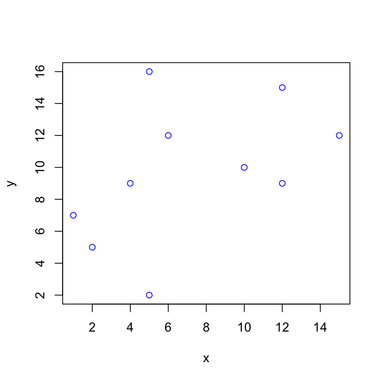
Given a list of cities, what is the shortest route that visits each city once and returns to the original city? This combinatorial optimization problem is the traveling salesman problem (TSP). When there are $K$ cities, the number of feasible solutions is equal to $(K-1)!/2$. It is difficult to enumerate and evaluate all solutions for a large number of cities. SA algorithm fits this problem quite well.
Let’s consider a toy problem with only 10 cities. To apply the SA algorithm, we need to determine a cooling schedule. For simplicity, we choose $T_k=T_0\alpha^k$. As for the energy function, the length of the route is a natural choice. For many problems, the challenge to apply SA is how to generate new solution from the incumbent. And most of the times there are various ways to do that, but some of which may not be efficient. In this TSP problem, we adopt a simple strategy, i.e., randomly select two different cities from the current route and switch them. If the switch results in a shorter route we would accept the switch; if the new route is longer, we sill could accept the switch with the acceptance probability.
The implementation of SA with this simple strategy is implemented in both R/Python as follows.
chapter5/TSP.R
 1 library(R6)
 2
 3 TSP = R6Class(
 4   "TSP",
 5   public = list(
 6     cities = NULL,
 7     distance = NULL,
 8     initialize = function(cities, seed = 42) {
 9       set.seed(seed)
10       self$cities = cities
11       self$distance = as.matrix(dist(cities))
12     },
13     calculate_length = function(path) {
14       l = 0.0
15       for (i in 2:length(path)) l = l+self$distance[path[i-1], path[i]]
16       l + self$distance[path[1],path[length(path)]]
17     },
18     accept = function(T_k, energy_old, energy_new) {
19       delta = energy_new - energy_old
20       p = exp(-delta/T_k)
21       p>=runif(1)
22     },
23     solve = function(T_0, alpha, max_iter) {
24       T_k = T_0
25       # create the initial solution s0
26       s = sample(nrow(self$distance), nrow(self$distance), replace=FALSE)
27       length_old = self$calculate_length(s)
28       for (i in 1:max_iter){
29         T_k = T_k*alpha
30         # we randomly exchange 2 cities in the route
31         candidates = sample(nrow(self$distance), 2, replace=FALSE)
32         temp = s[candidates[1]]
33         s[candidates[1]] = s[candidates[2]]
34         s[candidates[2]] = temp
35         length_new = self$calculate_length(s)
36         # check if we accept or reject the exchange
37         if (self$accept(T_k, length_old, length_new)){
38           # accept
39           length_old = length_new
40         }else{
41           # reject
42           s[candidates[2]] = s[candidates[1]]
43           s[candidates[1]] = temp
44         }
45       }
46       if (s[1]==1) return(list('s'=s,'length'=length_old))
47       start = which(s==1)
48       s_reordered = c(s[start:length(s)], s[1:start-1])
49       list('s'=s_reordered,'length'=length_old)
50     }
51   )
52 )
chapter5/TSP.py
 1 import numpy as np
 2 from scipy.spatial.distance import cdist
 3
 4 class TSP:
 5     def __init__(self, cities, seed=42):
 6         np.random.seed(seed)
 7         self.cities = cities
 8         # let's calculate the pairwise distance
 9         self.distance = cdist(cities, cities)
10
11     def calculate_length(self, path):
12         l = 0.0
13         for i in range(1, len(path)):
14             l += self.distance[path[i-1], path[i]]
15         return l + self.distance[path[-1], path[0]]
16
17     def accept(self, T_k, energy_old, energy_new):
18         delta = energy_new - energy_old
19         p = np.exp(-delta/T_k)
20         return p >= np.random.uniform(low=0.0, high=1.0, size=1)[0]
21
22     def solve(self, T_0, alpha, max_iter):
23         T_k = T_0
24         # let's create an initial solution s0
25         s = np.random.permutation(len(self.cities))
26         length_old = self.calculate_length(s)
27         for i in range(max_iter):
28             T_k *= alpha
29             # we randomly choose 2 cities and exchange their positions in the route
30             pos_1, pos_2 = np.random.choice(len(s), 2, replace=False)
31             s[pos_1], s[pos_2] = s[pos_2], s[pos_1]
32             length_new = self.calculate_length(s)
33             # check if we want to accept the new solution or not
34             if self.accept(T_k, length_old, length_new):
35                 # we accept the solution and update the old energy
36                 length_old = length_new
37             else:
38                 # we reject the solution and reverse the switch
39                 s[pos_1], s[pos_2] = s[pos_2], s[pos_1]
40         # let's reorder the result
41         if s[0] == 0:
42             return s, length_old
43         start = np.argwhere(s == 0)[0, 0]
44         return np.hstack((s[start:], s[:start])), length_old
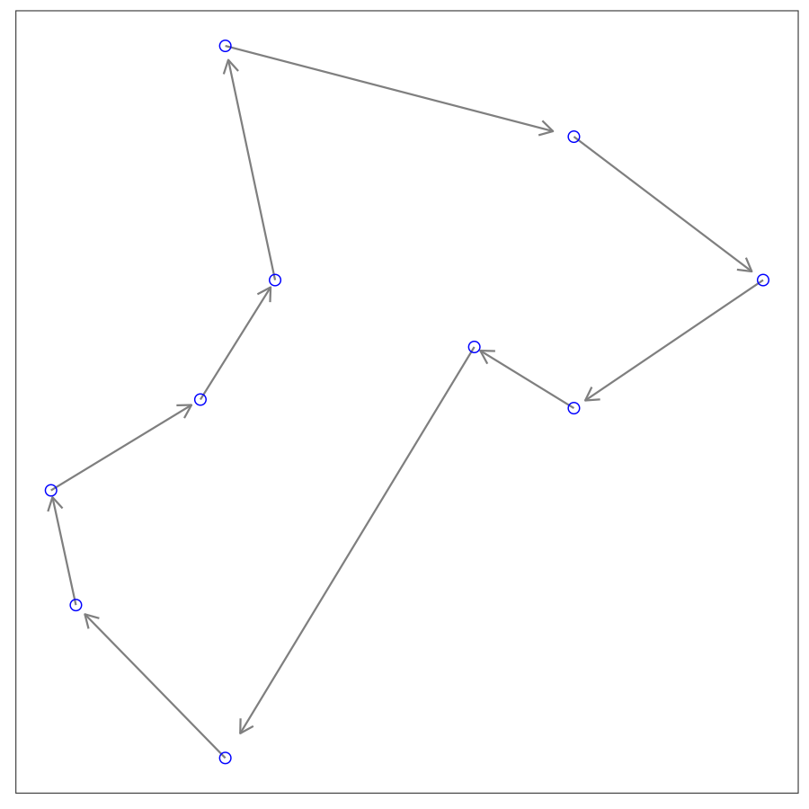
Let’s run our TSP solver to see the results.
1 > cities = read.csv( 'chapter5/cities.csv')
2 > cities = cities[,c('x','y')]
3 > tsp = TSP$new(cities)
4 > tsp$solve(2000,0.99,2000)
5 $s
6  [1]  1  3  2 10  5  6  9  4  7  8
7
8 $length
9 [1] 47.372551 >>> from TSP import TSP
2 >>> cities = pd.read_csv( 'chapter5/cities.csv')
3 >>> cities = list(zip(cities.x, cities.y))
4 >>> tsp = TSP(cities)
5 >>> tsp.solve(2000, 0.99, 2000)
6 (array([1, 2, 0, 7, 6, 3, 8, 5, 4, 9]), 47.372551972154646)In the implementation above, we set the initial temperature to $2000$, the cooling rate $\alpha$ to $0.99$. After 2000 iterations, we get the same routes from both implementations. In practice, it’s common to see metaheuristic algorithms get trapped in local optimums.
1 https://en.wikipedia.org/wiki/Operations_research
2 Stephen Boyd and Lieven Vandenberghe. Convex optimization. Cambridge university press, 2004.
3 https://en.wikipedia.org/wiki/Norm_(mathematics)
4 https://en.wikipedia.org/wiki/Efficient_estimator
5 Jerome Friedman, Trevor Hastie, and Robert Tibshirani. The elements of statistical learning. Springer series in statistics New York, NY, USA:, second edition, 2009.
6 Neal Parikh, Stephen Boyd, et al. Proximal algorithms. Foundations and Trends in Optimization, 1(3): 127–239, 2014.
7 https://en.wikipedia.org/wiki/Quasi-Newton_method
8 https://en.wikipedia.org/wiki/Nelder-Mead_method
9 https://en.wikipedia.org/wiki/Maximum_likelihood_estimation
10 George Casella and Roger L Berger. Statistical inference, volume 2. Duxbury Pacific Grove, CA, 2002.
11 https://archive.ics.uci.edu/ml/datasets/banknote+authentication
12 https://en.wikipedia.org/wiki/Linear_programming
13 George Dantzig. Linear programming and extensions. Princeton university press, 2016.
14 https://developers.google.com/optimization
15 https://scipy.org
16 https://www.cvxpy.org
17 https://cran.r-project.org/web/packages/lpSolve/lpSolve.pdf
18 https://en.wikipedia.org/wiki/Least_absolute_deviations
19 Jerome Friedman, Trevor Hastie, and Rob Tibshirani. glmnet: Lasso and elastic-net regularized gener- alized linear models. R package version, 1(4), 2009.
20 https://en.wikipedia.org/wiki/Quadratic_programming
21 https://cran.r-project.org/web/views/Optimization.html
22 Peter JM Van Laarhoven and Emile HL Aarts. Simulated annealing. In Simulated annealing: Theory and applications, pages 7–15. Springer, 1987.
23 https://en.wikipedia.org/wiki/Integer_programming