Another Book on Data Science - Machine Learning

Sections in this Chapter:

Supervised learning
Gradient boosting machine
Unsupervised learning
Reinforcement learning
Deep Q-networks
Computational differentiation

Machine learning is such a huge topic that we would only touch on a bit in this book. There are different learning paradigms.

Basically, supervised learning refers the learning task in which we have input data and output data and the purpose is to learn a functional map from the input data to the output data. In contrast to supervised learning, there is unsupervised learning in which only the input data in available. In addition to supervised/unsupervised learning, there are also other learning paradigms, such as reinforcement learning ²⁰ and transfer learning ²¹.

The is no strict distinction between different learning paradigms. For example, semi-supervised learning ²² falls between supervised learning and unsupervised learning, and supervised learning paradigm can also be found inside some modern reinforcement learning algorithms.

Supervised learning

In this book, we have talked about quite a few supervised learning models, such as linear regression and its variants, logistic regression. We will also spend some effort in tree-based models in this chapter. There are many other interest supervised learning models that we don’t cover in this book, such as support vector machine ²³, linear discriminant analysis ²⁴. Almost all well-known supervised learning models’ implementations can be found online and I recommend learning from reading the source code. As for the usage, there is an abundance of off-the-shelf options in both R and Python. Algorithm-wise, my favorite supervised learning models include linear models, gradient boosting trees, and (deep) neural network models. Linear models are simple with great interpretability; and it is rare if gradient boosting tree models or deep neural network models cannot match the prediction accuracy of other models for a specific problem.

Population & random sample

A population is a complete set of elements of interest for a specific problem. It is usually defined by the researcher of the problem. A population can be either finite or infinite. For example, if we define the set of real numbers as our population, it is infinite. But if we are only interested in the integers between 1 and 100, then we get a finite population.

A random sample is a set of elements selected from a population. The size of a random sample could be larger than the population since an element can be taken multiple times.
Why do we care random samples? Because we are interested in the population from which the random sample is taken, and the random sample could help to make inference on the population.

In predictive modeling, each element in the population has a set of attributes which are usually called features or covariates, as well as a label. For example, a bank may use the mortgage applicant’s personal information (FICO score, years of employment, debt to income ratio, etc.) as the covariates, and the status of the mortgage (default, or paid off) as the label. A predictive model can be used to predict the final status of the mortgage for a new applicant, and such kind of models are classification models. When a mortgage is in default status, the applicant may have already made payments partially. Thus, a model to predict the amount of loss for the bank is also useful, and such kind of models are regression models.

But why do we need a predictive model? If we know the labels of the entire population, nothing is needed to learn. All what we need is a database table or a dictionary (HashMap) for lookup. The issue is that many problems in the real world don’t allow us to have the labels of the entire population. And thus, we need to learn or infer based on the random sample collected from the unknown population.

Universal approximation & overfitting

Universal approximation

The Universal approximation theorem says that a single hidden layer neural network can approximate any continuous functions ($\mathbf{R}^n\rightarrow\mathbf{R}$) with sufficient number of neurons under mild assumptions on the activation function (for example, the sigmoid activation function)¹. There are also other universal approximators, such as the decision trees.

Not all machine learning models can approximate universally, for example, the linear regression without polynomial items. If we have the data from the entire population, we may fit the population with a universal approximator. But as we have discussed earlier, when the entire population is available there is no need to fit a machine learning model for prediction. But if only a random sample is available, is a universal approximator still the best choice? It depends.

Overfitting & cross-validation

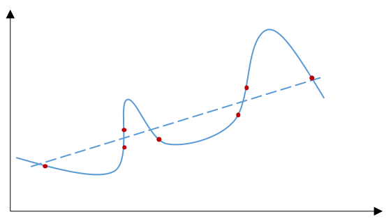
One of the risks of fitting a random sample with a predictive model is overfitting (see the figure below). Using universal approximators as the predictive model may even amplify such risk.

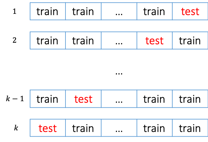
A random sample from a population that follows a linear model (the dashed line) is overfit by the solid curve.

To mediate the risk of overfitting, we usually use cross-validation to assess how accurately a predictive model is able to predict for unseen data. The following steps specifies how to perform a cross-validation.

divide the training data into $k$ partitions randomly
for $i=1,…,k$
- train a model using all partitions except partition $i$
- record the prediction accuracy of the trained model on partition $i$
calculate the average prediction accuracy.

Cross-validation can also be considered as a metaheuristic algorithm since it is not problem-specific because it doesn’t matter what type of predictive models we use.

There are some ready-to-use tools in R and Python modules for cross-validation. But for pedagogical purpose, let’s do it step by step. We do the cross validation using the Lasso regression we build in previous Chapter on the Boston dataset.

 1 source('../chapter5/lasso.R')
 2 
 3 library(caret)
 4 library(MASS)
 5 library(Metrics) # we use the rmse function from this package
 6 k = 5
 7 
 8 set.seed(42)
 9 # if we set returnTrain = TRUE, we get the indices for train partition
10 test_indices = createFolds(Boston$medv, k = k, list = TRUE, returnTrain = FALSE)
11 scores = rep(NA, k)
12 
13 for (i in 1:k){
14   lr = Lasso$new(200)
15   # we exclude the indices for test partition and train the model
16   lr$fit(data.matrix(Boston[-test_indices[[i]], -ncol(Boston)]), Boston$medv[-test_indices[[i]]], 100)
17   y_hat = lr$predict(data.matrix(Boston[test_indices[[i]], -ncol(Boston)]))
18   scores[i] = rmse(Boston$medv[test_indices[[i]]], y_hat)
19 }
20 print(mean(scores))

Python

 1 import sys
 2 sys.path.append("..")
 3 
 4 from sklearn.metrics import mean_squared_error
 5 from sklearn.datasets import load_boston
 6 from sklearn.model_selection import KFold
 7 from chapter5.lasso import Lasso
 8 
 9 
10 boston = load_boston()
11 X, y = boston.data, boston.target
12 
13 # create the partitions with k=5
14 k = 5
15 kf = KFold(n_splits=k)
16 # create a placeholder for the rmse on each test partition
17 scores = []
18 
19 for train_index, test_index in kf.split(X):
20     X_train, X_test = X[train_index], X[test_index]
21     y_train, y_test = y[train_index], y[test_index]
22     # let's train the model on the train partitions
23     lr = Lasso(200.0)
24     lr.fit(X_train, y_train, max_iter=100)
25     # now test on the test partition
26     y_hat = lr.predict(X_test)
27     # we calculate the root of mean squared error (rmse)
28     rmse = mean_squared_error(y_test, y_hat) ** 0.5
29     scores.append(rmse)
30 
31 # average rmse from 5-fold cross-validation
32 print(sum(scores)/k)

Run the code snippets, we have the $5$-fold cross-validation accuracy as follows.

1 chapter7 $r -f cv.R
2 [1] 4.978324

Python

1 chapter7 $python3.7 cv.py
2 5.702339699398128

We add the line sys.path.append("..") in the Python code, otherwise it would throw an error because of the import mechanism².

Evaluation metrics

In the example above, we measure the root of mean squared error (RMSE) as the accuracy of the linear regression model. There are various metrics to evaluate the accuracy of predictive models.

Metrics for regression

For regression models, RMSE, mean absolute error (MAE)³ and mean absolute percentage error (MAPE)⁴ are some of the commonly-used evaluation metrics. You may have heard of the coefficient of determination ($R^2$ or adjusted $R^{2}$) in Statistics. But from predictive modeling perspective, $R^{2}$ is not a metric that evaluates the predictive power of the model since its calculation is based on the training data. But what we are actually interested in is the model performance on the unseen data. In Statistics, goodness of fit is a term to describe how good a model fits the observations, and $R^{2}$ is one of these measures for goodness of fit. In predictive modeling, we care more about the error of the model on the unseen data, which is called generalization error. But of course, it is possible to calculate the counterpart of $R^{2}$ on testing data.

Some metrics for regression models

metric	formula
RMSE	$\sqrt{\frac {\sum_{i=1}^{n} {(\hat{y}_{i}-y})^{2}} n}$
MAE	$ \frac {\sum_{i=1}^{n} {\lvert \hat{y}_{i} – y \rvert}} {n} $
MAPE	$ \frac {1} n \sum_{i=1}^{n} \lvert{\frac {\hat{y}_{i}-y_{i}} {y_{i}}\rvert}$

Metrics for classification

The most intuitive metric for classification models is the accuracy, which is the percentage of corrected classified instances. To calculate the accuracy, we need to label each instance to classify. Recall the logistic regression we introduced in Chapter 5, the direct output of a logistic regression are probabilities rather than labels. In that case, we need to convert the probability output to the label for accuracy calculation. For example, consider a classification problem, where the possible labels of each instance is $0$, $1$, $2$ and $3$. If the predictive probabilities of each label are $0.2$, $0.25$, $0.5$, $0.05$ for label $0$, $1$, $2$ and $3$ respectively, then the predictive label is $2$ since its corresponding probability is the largest.

But actually we don’t always care the labels of an instance. For example, a classification model for mortgage default built in a bank may only be used to calculate the expected monetary loss. Another example is the recommendation system that predicts the probabilities which are used for ranking of items. In that case, the model performance could be evaluated by logloss, AUC, etc. using the output probabilities directly. We have seen in Chapter 5 the loss function of logistic regression is the log-likelihood function.

Actually, logloss is just the average evaluated log-likelihood on the testing data, and thus it can also be used for classification models with more than 2 classes (labels) because likelihood function is not restricted to Bernoulli distribution (extended Bernoulli distribution is called categorical distribution⁵). Another name of logloss is cross-entropy loss.

In practice, AUC (Area Under the ROC Curve) is a very popular evaluation metric for binary-class classification problems. AUC is bounded between 0 and 1. A perfect model leads to an AUC equal to 1. If a model’s predictions are $100\%$ wrong, the resulted AUC is equal to 0. But if we know a binary-class classification model always results in $100\%$ wrong predictions, we can instead use $1-\hat{y}$ as the corrected prediction and as a result we will get a perfect model and the AUC based on the corrected prediction becomes 1. Actually, a model using completely random guess as the prediction leads to an AUC equal to 0.5. Thus, in practice the evaluated AUC is usually between 0.5 and 1.

There are also many other metrics, such as recalls, precisions, and F1 score⁶.

The selection of evaluation metrics in predictive modeling is important but also subjective. Sometimes we may also need to define a customized evaluation metric.

Many evaluation metrics can be found from the R package Metrics and the Python module sklearn.metrics.

 1 > set.seed(42)
 2 > # regression metrics
 3 > y = rnorm(n = 10, mean = 10, sd = 2)
 4 > y
 5  [1] 12.741917  8.870604 10.726257 11.265725 10.808537  9.787751
 6  [7] 13.023044  9.810682 14.036847  9.874572
 7 > # we use random numbers as the predictions
 8 > y_hat = rnorm(n = 10, mean = 10.5, sd = 2.2) 
 9 > y_hat
10  [1] 13.370713 15.530620  7.444506  9.886665 10.206693 11.899091
11  [7]  9.874644  4.655798  5.130973 13.404249
12 > 
13 > rmse(actual = y, predicted = y_hat)
14 [1] 4.364646
15 > mae(actual = y, predicted = y_hat)
16 [1] 3.540164
17 > mape(actual = y, predicted = y_hat)
18 [1] 0.3259014
19 > # classification metrics
20 > y = rbinom(n = 10, size = 1, prob=0.25)
21 > y
22  [1] 0 0 0 1 0 1 1 0 1 0
23 > y_hat = runif(10, 0, 1)
24 > logLoss(y, y_hat)
25 [1] 0.4553994
26 > auc(y, y_hat)
27 [1] 0.8333333

Python

 1 >>> import numpy as np 
 2 >>> from sklearn.metrics import mean_squared_error, mean_absolute_error, log_loss, roc_auc_score
 3 >>> np.random.seed(42)
 4 >>> # regression metrics
 5 ... 
 6 >>> y = np.random.normal(10, 2, 10)
 7 >>> y_hat = np.random.normal(10.5, 2.2, 10)
 8 >>> mean_squared_error(y, y_hat) ** 0.5 # rmse
 9 3.0668667318485165
10 >>> mean_absolute_error(y, y_hat) # mae
11 2.1355703394788237
12 >>> # let's define mape since it's not available
13 ... 
14 >>> def mape(y, y_hat): return np.mean(np.abs(y-y_hat)/y_hat)
15 ...
16 >>> mape(y, y_hat)
17 0.292059554974094
18 >>> # classification metrics
19 >>> y = np.random.binomial(1, 0.25, 10)
20 >>> y_hat = np.random.uniform(0, 1, 10)
21 >>> log_loss(y, y_hat)
22 0.47071363776285635
23 >>> roc_auc_score(y, y_hat) # auc
24 0.8095238095238095

Feature engineering & embedding

According to the explanation of feature engineering⁷ on wikipedia, feature engineering is the process to use domain knowledge to create new features based on existing features. In reality, it is not rare to see feature engineering leads to better prediction accuracy. And sometimes I use feature engineering too. But I think feature engineering should be less and less useful in the future as the machine learning algorithms become more and more intelligent.

Let’s consider three features $x_{1},x_{2}$ and $x_{3}$ and assume the actual model is specified as $y=f(x_{1},g(x_{2}, x_{3}))$. After all, $y$ is still a function of $x_{1},x_{2}$ and $x_{3}$, and we can write it as $y=h(x_{1},x_{2}, x_{3})$. Thus, even without creating the new feature $x_{4}=g(x_{2}, x_{3})$ explicitly, a universal approximator should be able to learn (i.e., approximate) the function $h$ from the data ideally. This idea is also supported by the Kolmogorov–Arnold representation theorem⁸ which says any continuous real-valued multivariate functions can be written as a finite composition of continuous functions of a single variable.

$$
\begin{equation}
f(x\sb{1},…,x\sb{m})=\sum_{q=0}^{2m} {\Phi\sb{q}\big(\sum_{p=1} ^{m} \phi_{q,p} (x_{p})}\big) .
\label{eq:ka}
\end{equation}
$$

As of today, since the machine learning algorithms are not that intelligent, it is worth trying feature engineering especially when domain knowledge is available.

If you are familiar with dimension reduction, embedding can be considered as something similar. Dimension reduction aims reducing the dimension of $\boldsymbol{X}$. It sounds interesting and promising if we can transform the high-dimensional dataset into a a low-dimensional dataset and feed the dataset in a low dimension space to the machine learning model. However, I don’t think this is a good idea in general because it is not guaranteed the low-dimensional predictors still keep all the information related to the response variable. Actually, many machine learning models are capable to handle the high-dimensional predictors directly.

Embedding also transform the features into a new space, which usually has a lower dimension. But generally embedding is not done by the traditional dimension reduction techniques (for example, principal component analysis). In natural language process, a word can be embedded into a vector space by word2vec⁹ (or other techniques). When an instance is associated with an image, we may consider to use autoencoder¹⁰ to encode/embed the image into a space with lower dimension, which is usually achieved by (deep) neural networks.

Collinearity

Collinearity is one of the cliches in machine learning. For non-linear models, collinearity is usually not a problem. For linear models, I recommend reading this discussion¹¹ to see when it is not a problem.

Feature selection & parameter tuning

We have seen how the Lasso solutions of linear models can be used for feature selection in Chapter 5. What about non-linear models? There are some model-specific techniques for feature selection. Also, there is a metaheuristic approach to select features – cross-validation. Specifically, we can try different combinations of the features and use cross-validation to select the set of features which results in the best cross-validation evaluation metric. However, the major problem of this approach is its efficiency. When the number of features is too large, it is impossible to try all different combinations with limited computational resources. Thus, it is better to use the model-specific feature selection techniques in practice.

To tune model parameters, such as the $\lambda$ in Lasso, we can also use cross-validation. But again, the efficiency is our major concern.

Can we have feature selection and parameter tuning done automatically? Actually, automated machine learning has been a hot research topic in both academia and industry.

Gradient boosting machine

Decision tree

A decision tree consists of a bunch of nodes. In a decision tree there is a node with no parent nodes, which is called root node. The node without any children is called leaf node.

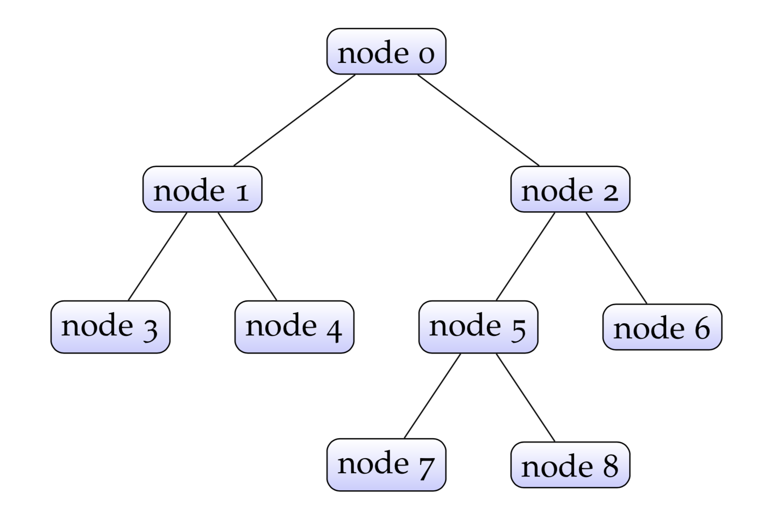
The length (number of nodes) of the longest path from the root node to a leaf node is called the depth of the tree. For example, the depth of the tree above is 4. Each leaf node has a label. In regression tasks, the label is a real number, and in classification tasks the label could could be a real number which is used to get the class indirectly (for example, fed into a sigmoid function to get the probability), or an integer representing the predicted class directly.

Each node except the leaves in a decision tree is associated with a splitting rule. These splitting rules determine to which leaf an instance belongs. A rule is just a function taking a feature as input and returns true or false as output. For example, a rule on the root could be $x_{1}<0$ and if it is true, we go to the left node otherwise go to the right node. Once we arrive at a leaf, we can get the predicted value based on the label of the leaf.

To get a closer look, let’s try to implement a binary tree structure for regression tasks in R/Python from scratch.

Let’s implement the binary tree as a recursive data structure, which is composed partially of similar instances of the same data structure. More specifically, a binary tree can be decomposed into three components, i.e., its root node, the left subtree under the root, and the right subtree of the root. To define a binary (decision) tree, we only need to define these three components. And to define the left and right subtrees, this decomposition is applied recursively until the leaves.

Now we have the big picture how to define a binary tree. However, to make the binary tree a decision tree, we also need to define the
splitting rules. For simplicity, we assume there is no missing value in our data and all variables are numeric. Then a splitting rule of a node is composed of two components, i.e., the variable to split on, and the corresponding breakpoint for splitting.

There is one more component we need to define in a decision tree, that is, the predict method which takes an instance as input and returns the prediction.

Now we are ready to define our binary decision tree.

chapter7/tree.R

  3   4   5   6   7   8   9  10  11  12  13  14  15  16  17  18  19  20  21  22  23  24  25  26  27  28  29  30  31  32  33  34  35  36  37  38  39  40  41  42  43  44  45  46  47  48  49  50  51  52  53  54  55  56  57  58  59  60  61

class="language-r" data-lang="r"> 1 library(R6) 2 Tree = R6Class( "Tree", public = list( left = NULL, right = NULL, variable_id = NULL, break_point = NULL, val = NULL, initialize = function(left, right, variable_id, break_point, val) { self$left = left self$right = right self$variable_id = variable_id self$break_point = break_point self$val = val }, is_leaf = function() { is.null(self$left) && is.null(self$right) }, depth = function() { if (self$is_leaf()) { 1 } else if (is.null(self$left)) { 1 + self$right$depth() } else if (is.null(self$right)) { 1 + self$left$depth() } else{ 1 + max(self$left$depth(), self$right$depth()) } }, predict_single = function(x) { # if x is a vector if (self$is_leaf()) { self$val } else{ if (x[self$variable_id] < self$break_point) { self$left$predict_single(x) } else{ self$right$predict_single(x) } } }, predict = function(x) { # if x is an array preds = rep(0.0, nrow(x)) for (i in 1:nrow(x)) { preds[i] = self$predict_single(x[i, ]) } preds }, print = function() { # we can call print(tree), similar to the magic method in Python cat("variable_id:", self$variable_id, "\n") cat("break at:", self$break_point, "\n") cat("is_leaf:", self$is_leaf(), "\n") cat("val:", self$val, "\n") cat("depth:", self$depth(), "\n") invisible(self) } ) )

Python

chapter7/tree.py

 1 class Tree:
 2     def __init__(self, left, right, variable_id, break_point, val):
 3         self.left = left
 4         self.right = right
 5         self.variable_id = variable_id
 6         self.break_point = break_point
 7         self.val = val
 8 
 9     @property
10     def is_leaf(self):
11         return self.left is None and self.right is None
12 
13     def _predict_single(self, x):
14         if self.is_leaf:
15             return self.val
16         if x[self.variable_id] < self.break_point:
17             return self.left._predict_single(x)
18         else:
19             return self.right._predict_single(x)
20 
21     def predict(self, x):
22         return [self._predict_single(e) for e in x]
23 
24     @property
25     def depth(self):
26         if self.is_leaf:
27             return 1
28         elif self.left is None:
29             return 1 + self.right.depth
30         elif self.right is None:
31             return 1 + self.left.depth
32         return 1 + max(self.left.depth, self.right.depth)
33 
34     def __repr__(self):
35         return "variable_id: {0}\nbreak_at: {1}\nval: {2}\nis_leaf: {3}\nheight: {4}".format(
36             self.variable_id, self.break_point, self.val, self.is_leaf, self.depth)

You may have noticed the usage @property in our Python implementation. It is one of builtin decorators in Python. We won’t talk too much of decorators. Basically, adding this decorator makes the method depth behave like a property, in the sense that we can call self.depth instead of self.depth() to get the depth.

In the R implementation, the invisible(self) is returned in the print method which seems strange. It is an issue¹² of R6 class due to the S3 dispatch mechanism which is not introduced in this book.

The above implementation doesn’t involve the training or fitting of the decision tree. In this book, we wouldn’t talk about how to fit a traditional decision tree model due to its limited usage in the context of modern machine learning. Let’s see how to use the decision tree structures we defined above by creating a pseudo decision tree illustrated below.

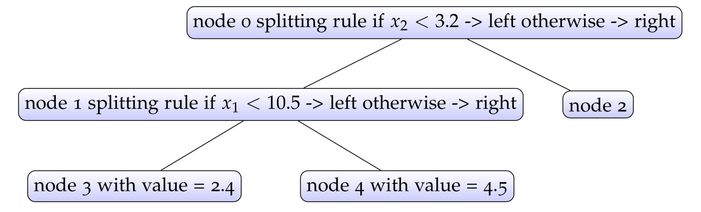
 1 > source('tree.R')
 2 > node_2 = Tree$new(NULL, NULL, NULL, NULL, 0.6)
 3 > node_3 = Tree$new(NULL, NULL, NULL, NULL, 2.4)
 4 > node_4 = Tree$new(NULL, NULL, NULL, NULL, 4.5)
 5 > node_1 = Tree$new(node_3, node_4, 1, 10.5, NULL)
 6 > node_0 = Tree$new(node_1, node_2, 2, 3.2, NULL)
 7 > print(node_0)
 8 variable_id: 2 
 9 break at: 3.2 
10 is_leaf: FALSE 
11 val: 
12 depth: 3 
13 > print(node_4)
14 variable_id: 
15 break at: 
16 is_leaf: TRUE 
17 val: 4.5 
18 depth: 1 
19 > x = array(c(10, 0.5), c(1, 2))
20 > node_0$predict(x)
21 [1] 2.4

Python

 1 >>> from tree import Tree
 2 >>> node_2 = Tree(None, None, None, None, 0.6)
 3 >>> node_3 = Tree(None, None, None, None, 2.4)
 4 >>> node_4 = Tree(None, None, None, None, 4.5)
 5 >>> node_1 = Tree(node_3, node_4, 0, 10.5, None)
 6 >>> node_0 = Tree(node_1, node_2, 1, 3.2, None)
 7 >>> 
 8 >>> print(node_0)
 9 variable_id: 1
10 break_at: 3.2
11 val: None
12 is_leaf: False
13 depth: 3
14 >>> print(node_4)
15 variable_id: None
16 break_at: None
17 val: 4.5
18 is_leaf: True
19 depth: 1
20 >>> x = [[10, 0.5]]
21 >>> node_0.predict(x)
22 [2.4]

It’s worth noting decision trees can approximate universally.

Tree growing in gradient boosting machine

What is a gradient boosting machine (GBM) (or gradient boosting regression)? Essentially, a GBM is just a forest of decision trees.
If you have heard of random forest (RF), you may know that a random forest is also a bunch of trees. What is the difference between a GBM and RF?

Looking at the fitted trees from RF and GBM, there is no way to tell if the trees are fitted by a RF or a GBM. The major difference is how these trees are trained, rather than the trees themselves. A minor difference is how these trees are used for prediction. In many RF implementations, the prediction for an instance is the average prediction of each tree within the forest. If it is a classification task, there are two ways to get the final prediction – (a) predict the class with majority voting directly, i.e., the predicted class is the one with highest frequency among the predicted classes of all trees; (b) predict the probability based on the frequencies, for example, if among five trees there are three trees output class 1 then the predicted probability of class 1 is equal to $3/5$. In many GBM implementations, the prediction (for regression tasks) is the sum of the predictions of individual trees.

GBM fits trees sequentially, but RF fits trees independently. The obvious advantage of fitting trees independently is that it can be done in parallel. But accuracy-wise, GBM usually performs better according to my limited experience.

We have seen the structure of a single decision tree in GBM. Now it’s time to see how to get these trees fitted in GBM. Let’s start from the first tree.

To grow a tree, we start from its root node. In GBM fitting, usually we pre-determine a maximum depth $d$ for each tree to grow. And the final tree’s depth may be equal to or less than the maximum depth $d$. At a high level, the tree is grown in a recursive fashion. Specifically, first we attempt to split the current node and if the splitting improves the performance we grow the left subtree and the right subtree under the root node. When we grow the left subtree, its maximum depth is $d-1$, and the same applies to the right subtree. We can define a tree grow function for such purpose which takes a root node $Node_{root}$ (it is also a leaf) as input. The pseudo code of tree grow function is illustrated below.

if $d>1$:
- call split function on $Node_{root}$
- if true is returned:
- call grow function on the empty $Node_{left}$ with $d-1$ maximum depth
- call grow function on the empty $Node_{right}$ with $d-1$ maximum depth
return

In fact, the algorithm of tree growing is just a DFS algorithm.

To complete the pseudo algorithm above, we need to have a split function which takes a leaf node as input and returns a boolean value as output. If true is returned, we will do the splitting, i.e., to grow the left/right subtree. So now the challenge is how to define the split function, which requires the understanding of the theories behind GBM.

Optimization of GBM

Similar to other regression models we have seen so far, GBM with $K$ trees has a loss function which is defined below.

$$
\begin{equation}
\mathcal{L}=\sum_{i=1}^{n} {(y_{i}-\hat{y}_{i})^{2}},
\label{eq:gbm0}
\end{equation}
$$
where

$$
\begin{equation}
\hat{y}_{i} = \sum_{t=1}^{K} {f_{t}(\boldsymbol{x}_{i})}.
\label{eq:treepred}
\end{equation}
$$

$f_{t}$ denotes the prediction of $t^{th}$ tree in the forest. As we mentioned previously, the fitting is done sequentially. When we fit the $t^{th}$ tree, all the previous $t-1$ trees are fixed. And the loss function for fitting the $t^{th}$ tree is given below.

$$
\begin{equation}
\mathcal{L}^{(t)}=\sum_{i=1}^{n} {(y_{i}- \sum_{l=1}^{t-1} {f_{l}(\boldsymbol{x}_{i})} – f_{t}(\boldsymbol{x}_{i}))^{2}}
\label{eq:gbm_t}
\end{equation}
$$

In practice, a regularized loss function \eqref{eq:treepred1} is used instead of \eqref{eq:treepred} to reduce overfitting.

$$
\begin{equation}
\mathcal{L}^{(t)}=\sum_{i=1}^{n} {(y_{i}- \sum_{l=1}^{t-1} {f_{l}(\boldsymbol{x}_{i})} – f_{t}(\boldsymbol{x}_{i}))^{2}} + \Phi(f_{t}).
\label{eq:treepred1}
\end{equation}
$$

Let’s follow the paper¹³ and use the number of leaves as well as the L2 penalty of the values (also called weights) of the leaves for regularization. The loss function then becomes

$$
\begin{equation}
\mathcal{L}^{(t)}=\sum_{i=1}^{n} {(y_{i}- \sum_{l=1}^{t-1} {f_{l}(\boldsymbol{x}_{i})} – f_{t}(\boldsymbol{x}_{i}))^{2}} + \gamma T + \frac 1 2 {\lambda \sum_{j=1}^{T}{\omega_{j}^{2}}} ,
\label{eq:growtree0}
\end{equation}
$$
where $\omega_{j}$ is the value associated with the $j_{th}$ leaf of the current tree.

Again, we get an optimization problem, i.e., to minimize the loss function \eqref{eq:growtree0}. The minimization problem can also be viewed as a quadratic programming problem. However, it seems different from the other optimization problems we have seen before, in the sense that the decision tree $f_{t}$ is a non-parametric model. A model is non-parametric if the model structure is learned from the data rather than pre-determined.

A common approach used in GBM is the second order approximation. By second order approximation, the loss function becomes

$$
\begin{equation}
\mathcal{L}^{(t)}\approx \sum_{i=1}^{n} {(y_{i} – \sum_{l=1}^{t-1} {f_{l}(\boldsymbol{x}_{i})})^2} + \sum_{i=1}^{n} {(g_{i}f_{t}(\boldsymbol{x}_{i}) +\frac 1 2 {h_{i}f_{t}(\boldsymbol{x}_{i})^{2}})} + \gamma T + \frac 1 2 {\lambda \sum_{j=1}^{T}{\omega_{j}^{2}}} ,
\label{eq:growtree}
\end{equation}
$$
where $g\sb{i}=2(f\sb{t}(\boldsymbol{x}\sb{i}) + \sum\sb{l=1}^{t-1} {f\sb{l}(\boldsymbol{x}_{i})} – y_{i})$ and $h\sb{i}=2$ are the first and the second order derivatives of the function $(y\sb{i}- \sum_{l=1}^{t-1} {f\sb{l}(\boldsymbol{x}\sb{i})-f\sb{t}(\boldsymbol{x}\sb{i}))^{2}} $ with respect to the function $f_{t}(\boldsymbol{x}_{i})$.

Let’s implement the function to calculate $g$ and $h$ and put them into util.py.

Python

chapter7/util.py

1 import numpy as np
2 
3 def gh_lm(actual, pred):
4     '''
5     gradient and hessian for linear regression loss
6     '''
7     return 2*(pred-actual), 2.0

Since the first item is a constant, let’s ignore it.

$$
\begin{equation}
\mathcal{L}^{(t)}\approx\sum_{i=1}^{n} {(g_{i}f_{t}(\boldsymbol{x}_{i}) +\frac 1 2 {h_{i}f_{t}(\boldsymbol{x}_{i})^{2}})} + \gamma T + \frac 1 2 {\lambda \sum_{j=1}^{T}{\omega_{j}^{2}}} ).
\label{eq:growtree1}
\end{equation}
$$

Let’s think of the prediction of an instance of the current tree. The training data, i.e., instances fall under the leaves of a tree. Thus, the prediction of an instance is the value $\omega$ associated with the corresponding leaf that the instance belongs to. Based on this fact, the loss function can be further rewritten as follows,

$$
\begin{equation}
\mathcal{L}^{(t)} \approx \sum\sb{j=1}^{T} {(\omega \sb{j} \sum\sb{i\in I\sb{j} }{g\sb{i}} + \frac 1 2 {\omega \sb{j} ^{2}( \sum\sb{i\in I\sb{j}} h\sb{i} +\lambda ) }}) + \gamma T .
\label{eq:growtree2}
\end{equation}
$$

When the structure of the tree is fixed the loss function \eqref{eq:growtree2} is a quadratic convex function of $\omega_{j}$, and the optimal solution can be obtained by setting the derivative to zero.

$$
\begin{equation}
\omega_{j}=- \frac {\sum_{i\in I_{j} } g_{i}} {\sum_{i\in I_{j}} h_{i} +\lambda}
\label{eq:omega}
\end{equation}
$$

Plugging \eqref{eq:omega} into the loss function results in the minimal loss of the current tree structure

$$
\begin{equation}
-\frac 1 2 \sum_{j=1}^{T} {\frac {(\sum_{i\in I_{j} }g_{i})^{2}} {\sum_{i\in I_{j}}h_{i} +\lambda} } + \gamma T .
\label{eq:minimalloss}
\end{equation}
$$

Now let’s go back to the split function required in the tree grow function discussed previously. How to determine if we need a splitting on a leaf? \eqref{eq:minimalloss} gives the solution – we can calculate the loss reduction after splitting which is given below

$$
\begin{equation}
\frac 1 2 {\bigg(\frac {(\sum\sb{i\in I\sb{left} }g\sb{i})^{2}} {\sum\sb{i\in I\sb{left}}h\sb{i}+ \lambda } + \frac {(\sum\sb{i\in I\sb{right} }g\sb{i})^{2}} {\sum\sb{i\in I\sb{right}}h\sb{i} + \lambda} – \frac {(\sum\sb{i\in I } g\sb{i})^{2}} {\sum\sb{i\in I} h\sb{i}+\lambda} \bigg)} – \gamma .
\label{eq:lossreduction}
\end{equation}
$$

If the loss reduction is positive, the split function returns true otherwise returns false.

So far, we have a few ingredients ready to implement our own GBM, which are listed below,

the structure of a single decision tree in the forest, i.e., the Tree class defined;
the node splitting mechanism, i.e., \eqref{eq:lossreduction};
the tree growing mechanism, i.e., the pseudo algorithm with the leaf value calculation \eqref{eq:omega}.

However, there are a few additional items we need to go through before the implementation.

In Chapter 6, we have seen how stochasticity works in iterative optimization algorithms. The stochasticity can be applied in both instance-wise and feature-wise. The stochasticity technique is very important is the optimization of GBM. More specifically, we apply the stochasticity both instance-wise and feature-wise. Instance-wise, when we fit a new tree, we randomly get a subsample from the training sample. And feature-wise, we randomly select a few features/variables when we fit a new tree. The stochasticity technique could help to reduce overfitting. The extent of the stochasticity can be controlled by arguments.

Like the gradient decent algorithm, in GBM there is also a learning rate parameter which scales the values of the leaves after a tree is fitted.

In practice, we may also not want to have too few instances under a leaf, to reduce potential overfitting. When there are two few instances under a leaf, we may just stop the splitting process.

Now we have almost all the ingredients to make a working GBM. Let’s define the split_node function in the code snippet below.

Python

chapter7/grow.py

  1 from tree import Tree
  2 import numpy as np
  3 import pdb
  4 
  5 
  6 def split_node(f_in_tree, x_in_node, x_val_sorted, x_index_sorted, g_tilde, h_tilde, lam, gamma, min_instances):
  7     '''
  8     f_in_tree: a list of booleans indicating which variable/feature is selected in the tree
  9     x_in_ndoe: a list of booleans indicating which instance is used in the tree
 10     x_val_sorted: a nested list, x_val_sorted[feature index] is a list of instance values 
 11     x_index_sorted: a nested list, x_index_sorted[feature index] is a list of instance indexes
 12     g_tilde: first order derivative
 13     h_tilde: second order derivative
 14     lam: lambda for regularization
 15     gamma: gamma for regularization
 16     min_instances: the minimal number of instances under a leaf
 17     at the beginning we assume all instances are on the right
 18     '''
 19     if sum(x_in_node) < min_instances:
 20         return False, None, None, None, None, None, None
 21     best_break = 0.0
 22     best_feature, best_location = 0, 0
 23     ncol, nrow = len(f_in_tree), len(x_in_node)
 24     g, h = 0.0, 0.0
 25     for i, e in enumerate(x_in_node):
 26         if e:
 27             g += g_tilde[i]
 28             h += h_tilde[i]
 29     base_score = g*g/(h+lam)
 30     score_reduction = -np.inf
 31     best_w_left, best_w_right = None, None
 32     for k in range(ncol):
 33         if f_in_tree[k]:
 34             # if the feature is selected for this tree
 35             best_n_left_k = 0
 36             n_left_k = 0
 37             # feature is in the current tree
 38             g_left, h_left = 0.0, 0.0
 39             g_right, h_right = g-g_left, h-h_left
 40             # score reduction for current feature k
 41             score_reduction_k = -np.inf
 42             for i in range(nrow):
 43                 # for each in sample, we try to split on it
 44                 index = x_index_sorted[k][i]
 45                 if x_in_node[index]:
 46                     n_left_k += 1
 47                     best_n_left_k += 1
 48                     g_left += g_tilde[index]
 49                     g_right = g-g_left
 50                     h_left += h_tilde[index]
 51                     h_right = h-h_left
 52                     # new score reduction
 53                     score_reduction_k_i = g_left*g_left/(h_left+lam) + \
 54                         (g_right*g_right)/(h_right+lam)-base_score
 55                     if score_reduction_k <= score_reduction_k_i:
 56                         best_n_left_k = n_left_k
 57                         best_break_k = x_val_sorted[k][i]
 58                         best_location_k = i
 59                         score_reduction_k = score_reduction_k_i
 60                         w_left_k = -g_left/(h_left+lam)
 61                         w_right_k = -g_right/(h_right+lam)
 62 
 63             # if the score reduction on feature k is a better candidate
 64             if score_reduction_k >= score_reduction:
 65                 score_reduction = score_reduction_k
 66                 best_feature = k
 67                 best_break = best_break_k
 68                 best_location = best_location_k
 69                 best_w_left = w_left_k
 70                 best_w_right = w_right_k
 71     return 0.5*score_reduction >= gamma, best_feature, best_break, best_location, best_w_left, best_w_right, score_reduction
 72 
 73 
 74 def grow_tree(current_tree, f_in_tree, x_in_node, max_depth, x_val_sorted, x_index_sorted, y, g_tilde, h_tilde, eta, lam, gamma, min_instances):
 75     '''
 76     current_tree: the current tree to grow, i.e., a node
 77     f_in_tree, x_in_node, x_val_sorted, x_index_sorted: see split_node function
 78     max_depth: maximinum depth to grow
 79     eta: learning rate
 80     y: the response variable
 81     '''
 82     nrow = len(y)
 83     if max_depth == 0:
 84         return
 85     # check if we need a split
 86     do_split, best_feature, best_break, best_location, w_left, w_right, _ = split_node(
 87         f_in_tree, x_in_node, x_val_sorted, x_index_sorted, g_tilde, h_tilde, lam, gamma, min_instances)
 88 
 89     if do_split:
 90         # update the value/weight with the learning rate eta
 91         w_left_scaled = w_left*eta
 92         w_right_scaled = w_right*eta
 93         current_tree.variable_id = best_feature
 94         current_tree.break_point = best_break
 95         current_tree.val = None
 96 
 97         # initialize the left subtree
 98         current_tree.left = Tree(None, None, None, None, w_left_scaled)
 99         # initialize the right subtree
100         current_tree.right = Tree(None, None, None, None, w_right_scaled)
101         # update if an instance is in left or right
102         x_in_left_node = [False]*len(x_in_node)
103         x_in_right_node = [False]*len(x_in_node)
104         for i in range(nrow):
105             index = x_index_sorted[best_feature][i]
106             if x_in_node[index]:
107                 if i <= best_location:
108                     x_in_left_node[index] = True
109                 else:
110                     x_in_right_node[index] = True
111         # recursively grow its left subtree
112         grow_tree(current_tree.left, f_in_tree, x_in_left_node, max_depth-1,
113                   x_val_sorted, x_index_sorted, y, g_tilde, h_tilde, eta, lam, gamma, min_instances)
114         # recursively grow its right subtree
115         grow_tree(current_tree.right, f_in_tree, x_in_right_node, max_depth-1,
116                   x_val_sorted, x_index_sorted, y, g_tilde, h_tilde, eta, lam, gamma, min_instances)
117     else:
118         # current node is a leaf, so we update the value/weight of the leaf
119         g, h = 0.0, 0.0
120         for i, e in enumerate(x_in_node):
121             if e:
122                 g += g_tilde[i]
123                 h += h_tilde[i]
124         w_left_scaled = -g/(h+lam)*eta
125         current_tree.val = w_left_scaled

And the implementation of the GBM class is given below.

Python

chapter7/gbm.py

 1 from tree import Tree
 2 from grow import grow_tree, split_node
 3 from utils import gh_lm, rmse
 4 import numpy as np
 5 
 6 
 7 class GBM:
 8     def __init__(self, x_train, y_train, depth, eta, lam, gamma, sub_sample, sub_feature, min_instances=2):
 9         '''
10         x_train, y_train: training data
11         depth: maximum depth of each tree
12         eta: learning rate
13         lam and gamma: regularization parameters
14         sub_sample: control the instance-wise stochasticity
15         sub_feature: control the feature-wise stochasticity
16         min_instances: control the mimimum number of instances under a leaf
17         '''
18         self.n = len(x_train)
19         self.m = len(x_train[0])
20         self.x_train = x_train
21         self.y_train = y_train
22         self.x_test, self.y_test = None, None
23         self.depth = depth
24         self.eta = eta
25         self.lam = lam
26         self.gamma = gamma
27         self.sub_sample = sub_sample
28         self.sub_feature = sub_feature
29         self.min_instances = min_instances
30 
31         self.y_tilde = [0]*len(y_train)
32         self.g_tilde, self.h_tilde = [0] * \
33             len(self.y_tilde), [0]*len(self.y_tilde)
34         for i in range(len(self.y_tilde)):
35             self.g_tilde[i], self.h_tilde[i] = gh_lm(
36                 y_train[i], self.y_tilde[i])
37         x_columns = x_train.transpose()
38         self.nf = min(self.m, max(1, int(sub_feature*self.m)))
39         self.x_val_sorted = np.sort(x_columns)
40         self.x_index_sorted = np.argsort(x_columns)
41         self.forest = []
42 
43     def set_test_data(self, x_test, y_test):
44         self.x_test = x_test
45         self.y_test = y_test
46 
47     def predict(self, x_new):
48         y_hat = np.array([0.0]*len(x_new))
49         for tree in self.forest:
50             y_hat += np.array(tree.predict(x_new))
51         return y_hat
52 
53     def fit(self, max_tree, seed=42):
54         np.random.seed(seed)
55         self.forest = []
56         i = 0
57         while i < max_tree:
58             # let's fit tree i
59             # instance-wise stochasticity
60             x_in_node = np.random.choice([True, False], self.n, p=[
61                                          self.sub_sample, 1-self.sub_sample])
62             # feature-wise stochasticity
63             f_in_tree_ = np.random.choice(
64                 range(self.m), self.nf, replace=False)
65             f_in_tree = np.array([False]*self.m)
66             for e in f_in_tree_:
67                 f_in_tree[e] = True
68             del f_in_tree_
69             # initialize the root of this tree
70             root = Tree(None, None, None, None, None)
71             # grow the tree from root
72             grow_tree(root, f_in_tree, x_in_node, self.depth-1, self.x_val_sorted,
73                       self.x_index_sorted, self.y_train, self.g_tilde, self.h_tilde, self.eta, self.lam, self.gamma, self.min_instances)
74             if root is not None:
75                 i += 1
76                 self.forest.append(root)
77             else:
78                 next
79             for j in range(self.n):
80                 self.y_tilde[j] += self.forest[-1]._predict_single(
81                     self.x_train[j])
82                 self.g_tilde[j], self.h_tilde[j] = gh_lm(
83                     self.y_train[j], self.y_tilde[j])
84             if self.x_test is not None:
85                 # test on the testing instances
86                 y_hat = self.predict(self.x_test)
87                 print("iter: {0:>4}   rmse: {1:1.6f}".format(
88                     i, rmse(self.y_test, y_hat)))

Now let’s see the performance of our GBM implemented from scratch.

Python

chapter7/test_gbm.py

 1 from gbm import GBM
 2 import numpy as np
 3 from sklearn import datasets
 4 from sklearn.utils import shuffle
 5 
 6 
 7 def get_boston_data(seed=42):
 8     boston = datasets.load_boston()
 9     X, y = shuffle(boston.data, boston.target, random_state=seed)
10     X = X.astype(np.float32)
11     offset = int(X.shape[0] * 0.8)
12     X_train, y_train = X[:offset], y[:offset]
13     X_test, y_test = X[offset:], y[offset:]
14     return X_train, y_train, X_test, y_test
15     
16 if __name__ == "__main__":
17     X_train, y_train, X_test, y_test = get_boston_data(42)
18     gbm = GBM(X_train, y_train, depth=6, eta=0.05, lam=1.0,
19               gamma=1, sub_sample=0.5, sub_feature=0.7)
20     gbm.set_test_data(X_test, y_test)
21     gbm.fit(max_tree=200)

Running the code above, we have output as below.

Python

 1 chapter7 $python3.7 test_gbm.py
 2 iter:    1   rmse: 23.063019
 3 iter:    2   rmse: 21.997972
 4 iter:    3   rmse: 21.026602
 5 iter:    4   rmse: 20.043397
 6 iter:    5   rmse: 19.210746
 7 ...
 8 iter:  196   rmse: 2.560747
 9 iter:  197   rmse: 2.544847
10 iter:  198   rmse: 2.541102
11 iter:  199   rmse: 2.537366
12 iter:  200   rmse: 2.535143

We don’t implement the model in R, but it is not difficult to do based on the Python implementation above.

GBM can be used with various loss functions, and the major difference is the implementation of the first/second order derivatives, i.e., $g$ and $h$.

Regardless of the performance, there are two major missing features in our implementation is a) cross-validation and b) early stopping.
We have talked about cross-validation, but what is early stopping? It is a very useful technique in GBM. Usually, the cross-validated loss decreases when we add new trees at the beginning and at a certain point, the loss may increase when more trees are fitted (due to overfitting). Thus, we may select the best number of trees based on the cross-validated loss. Specifically, stop the fitting process when the cross-validated loss doesn’t decrease. In practice, we don’t want to stop the fitting immediately when the cross-validated loss starts increasing. Instead, we specify a number of trees, e.g. 50, as a buffer, after which the fitting process should stop if cross-validated loss doesn’t decrease.

Early stopping is also used in other machine learning models, for example, neural network. Ideally, we would like to have early stopping based on the cross-validated loss. But when the training process is time-consuming, it’s fine to use the loss on a testing date set¹⁴.

The commonly used GBM packages include XGBoost¹⁵, LightGBM¹⁶ and CatBoost¹⁷.

Let’s see how to use XGBoost for the same regression task on the Boston dataset.

chapter7/xgb.R

 1 library(xgboost)
 2 library(MASS)
 3 library(Metrics)
 4 set.seed(42)
 5 train_index = sample(nrow(Boston), floor(0.8 * nrow(Boston)), replace = FALSE)
 6 Boston = data.matrix(Boston)
 7 target_col = which(colnames(Boston) == 'medv')
 8 X_train = Boston[train_index, -target_col]
 9 y_train = Boston[train_index, target_col]
10 X_test = Boston[-train_index, -target_col]
11 y_test = Boston[-train_index, target_col]
12 # prepare the data for training and testing
13 dTrain = xgb.DMatrix(X_train, label = y_train)
14 dTest = xgb.DMatrix(X_test)
15 params = list(
16   "booster" = "gbtree",
17   "objective" = "reg:linear",
18   "eta" = 0.1,
19   "max_depth" = 5,
20   "subsample" = 0.6,
21   "colsample_bytree" = 0.8,
22   "min_child_weight" = 2
23 )
24 # run the cross-validation
25 hist = xgb.cv(
26   params = params,
27   data = dTrain,
28   nrounds = 500,
29   early_stopping_rounds = 50,
30   metrics = 'rmse',
31   nfold = 5,
32   verbose = FALSE
33 )
34 # since we have the best number of trees from cv, let's train the model with this number of trees
35 model = xgb.train(params, nrounds = hist$best_iteration, data = dTrain)
36 pred = predict(model, dTest)
37 
38 cat(
39   "rmse on testing instances is",
40   rmse(y_test, pred),
41   "with",
42   hist$best_iteration,
43   "trees"
44 )

Python

chapter7/xgb.py

 1 import xgboost as xgb
 2 from sklearn import datasets
 3 from sklearn.utils import shuffle
 4 from sklearn.metrics import mean_squared_error
 5 import numpy as np
 6 
 7 seed = 42
 8 boston = datasets.load_boston()
 9 X, y = shuffle(boston.data, boston.target, random_state=seed)
10 X = X.astype(np.float32)
11 offset = int(X.shape[0] * 0.8)
12 X_train, y_train = X[:offset], y[:offset]
13 X_test, y_test = X[offset:], y[offset:]
14 
15 params = {'booster': 'gbtree', 'objective': 'reg:linear', 'learning_rate': 0.1,
16           'max_depth': 5, 'subsample': 0.6, 'colsample_bytree': 0.8, 'min_child_weight': 2}
17 
18 # prepare the data for training and testing
19 dtrain = xgb.DMatrix(data=X_train, label=y_train, missing=None)
20 dtest = xgb.DMatrix(X_test)
21 
22 # run 5-fold cross-validation with maximum 1000 trees, and try to minimize the metric rmse
23 # early stopping 50 trees
24 hist = xgb.cv(params, dtrain=dtrain, nfold=5,
25               metrics=['rmse'], num_boost_round=1000, maximize=False, early_stopping_rounds=50)
26 
27 # find the best number of trees from the cross-validation history
28 best_number_trees = hist['test-rmse-mean'].idxmin()
29 
30 # since we have the best number of trees from cv, let's train the model with this number of trees
31 model = xgb.train(params, dtrain, num_boost_round=best_number_trees)
32 pred = model.predict(dtest)
33 print(
34     f"rmse on testing instances is {mean_squared_error(pred, y_test)**0.5:.6f} with {best_number_trees} trees")

The parameters subsample and colsample_bytree control the stochasticity, within the range of $[0, 1]$. If we set these two parameters to 1, then all instances and all features are selected for fitting every tree.

The two code snippets illustrate a minimal workflow of fitting a GBM model. First, we conduct (hyper) parameter tuning (such as learning rate, number of trees, regularization parameters, stochasticity parameters) with cross-validation, and next we train the model with the tuned parameters.

Running the code snippets, we have the following results.

1 > source('xgb.R')
2 rmse on testing instances is 2.632298 with 83 trees

Python

1 chapter7 $python3.7 xgb.py
2 rmse on testing instances is 2.736038 with 179 trees

In XGBoost, we could also use linear regression models as the booster (or base learner) instead of decision trees. However, when 'booster':'gblinear' is used, the sum of the prediction from all boosters in the model is equivalent to the prediction from a single (combined) linear model. In that sense, what we get is just a Lasso solution of a linear regression model.

GBM can be used in different tasks, such as classification, ranking, survival analysis, etc. When we use GBM for predictive modeling, missing value imputation is not required, which is one big advantage over linear models. But in our own implementation we don’t consider missing values for simplicity. In GBM, if a feature is categorical we could do label-encoding¹⁸, i.e., mapping the feature to integers directly without creating dummy variables (such as one-hot encoding). Of course one-hot encoding¹⁹ can also be used. But when there are too many new columns created by one-hot encoding, the probability that the original categorical feature is selected is higher than these numerical variables. In other words, we are assigning a prior weight to the categorical feature regarding the feature-wise stochasticity.

For quite a few real-world prediction problems, the monotonic constraints are desired. Monotonic constraints are either increasing or decreasing. The increasing constraint for feature $x_k$ refer to the relationship that $f(x_1,…,x_k,…,x_m)\le f(x_1,…,x_k’,…,x_m)$ if $x_k\le x_k’$. For example, an increasing constraint for the number of bedrooms in a house price prediction model makes lots of sense. Using gradient boosting tree regression models we can enforce such monotonic constraints in a straightforward manner. Simply, after we get the best split for the current node, we may check if the monotonic constraint is violated by the split. The split won’t be adopted if the constraint is broken.

Unsupervised learning

For many supervised learning tasks, we could formulate the problem as an optimization problem by writing down the loss function as a function of training input and output. In unsupervised learning problems there are no label/output. It is more difficult to formulate unsupervised learning problems in a unified approach. Still, some unsupervised learning problems can still be formulated as an optimization problem. Let’s see a few examples briefly.

Principal component analysis (PCA)

PCA is a very popular technique in many Engineering disciplines. As you may heard of PCA, it is a technique for dimension reduction. More specific, let $\boldsymbol{x}$ denote a $n*m$ matrix, and each row of $\boldsymbol{x}$ denoted as $\boldsymbol{x_i}’$ represents a point in $\mathbb{R}^m$. Sometimes the dimension $m$ could be relatively large and we don’t like that. In order to represent the data in a more compact way, we want to transform the raw data points into a new coordinate system in $\mathbb{R}^p$ where $p<m$. The $k^{th};k=1,…,p$ coordinate of $\boldsymbol{x_i}$ in the new coordinate system can be written $\boldsymbol{w_k}’\boldsymbol{x_i}$. However, there are infinite $\boldsymbol{w_k}$ for the transformation and we have to make a guidance for such transformation. The key of our guidance is to make the data points projected onto the first transformed coordinate have the largest variance, and $\boldsymbol{w_1}’\boldsymbol{x_i}$ is called the first principal component. And we could find the remaining transformations and principal components iteratively.

So now we see how the PCA is formulated as an optimization problem. However, under the above setting, there are infinite solutions for $\boldsymbol{w_k}$. We usually add a constraint on $\boldsymbol{w_k}$ in PCA, i.e., $|\boldsymbol{w_k}|=1$. The solution to this optimization problem is surprisingly elegant – the optimal $\boldsymbol{w_k}$ is the eigen vectors of the covariance matrix of $\boldsymbol{x}$. Now let’s try to conduct a PCA with eigen decomposition (it can also be done with other decompositions).

 1 > set.seed(42)
 2 > n = 1000
 3 > # we simulate some data points on a 2d plane
 4 > x1 = rexp(n)
 5 > x2 = x1*3 + rnorm(n, 12, 2)
 6 > x = cbind(x1, x2)
 7 > # total marginal variance
 8 > sum(diag(cov(x)))
 9 [1] 15.54203
10 > pca_vectors = eigen(cov(x))$vectors
11 > # find the projection on the new coordinate system
12 > z = x %*% pca_vectors
13 > # total marginal variance after transformation
14 > sum(diag(cov(z)))
15 [1] 15.54203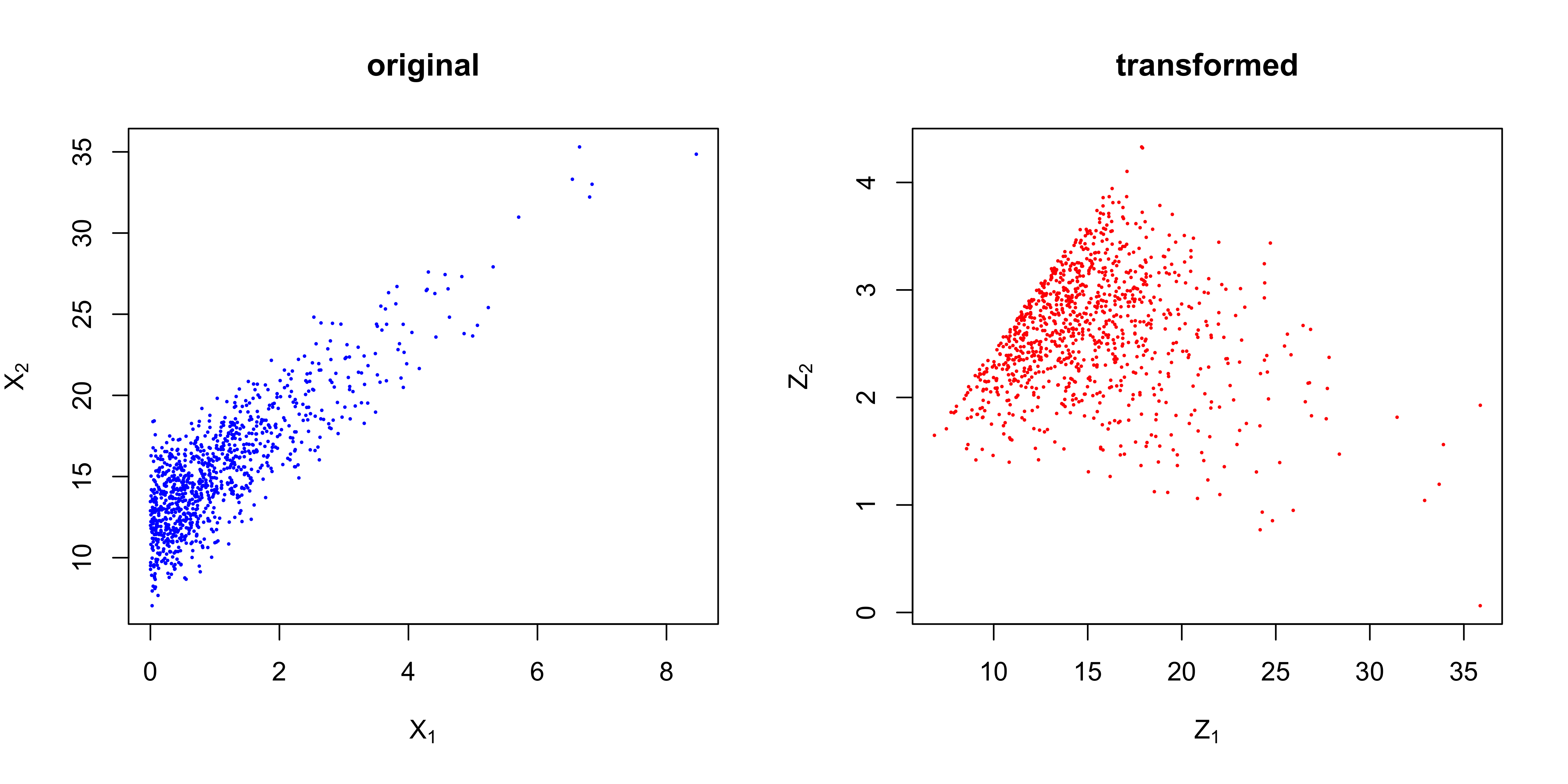

Original vs transformed data points via PCA

In fact, it does not matter if the raw data points are centered or not if the eigen decomposition is on the covariance matrix. If you prefer to decompose $\boldsymbol{x’}\boldsymbol{x}$ directly, centering is a necessary step. Many times, we don’t want to perform PCA in this way since there are a lot of functions/packages available in both R and Python.

Mixture model

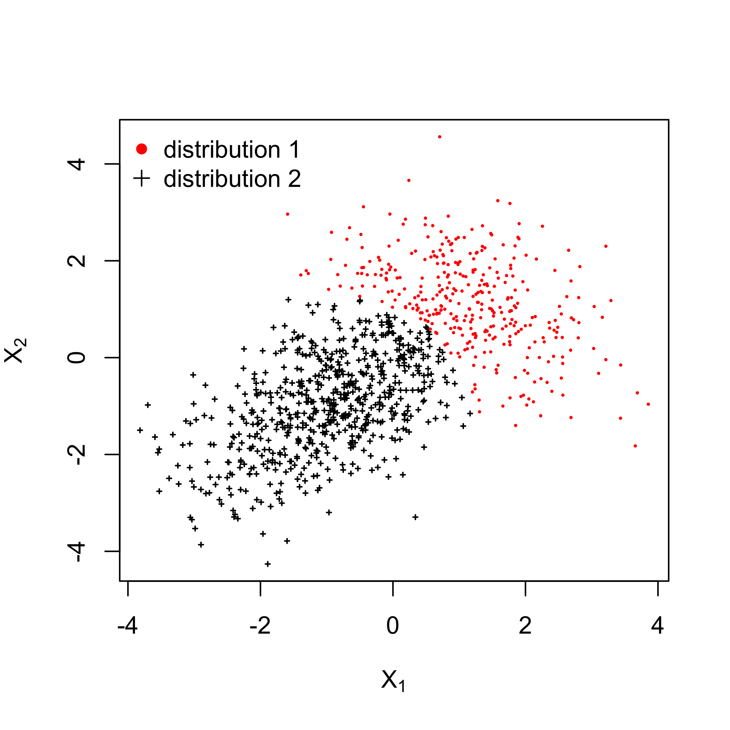
In previous chapters we have seen how to fit a distribution to data. What if the data points actually come from multiple distributions, for example, a mixture of two Gaussian distribution. If we know from which distribution each observed data point comes from it is not difficult to estimate the parameters. But in some situations it is impossible to tell the actual distribution a point is sampled from. Usually, a mixture of multiple distributions can be estimated by maximum likelihood method. We can derive the likelihood function of the observed data points and then we have an optimization problem.

Suppose we have a random size with sample size $n$, and each sample $x_i;i=1,…,n$ is from one of the $K$ multivariate Guassian distributions. The $k^{th}$ distribution is denoted as $\mathcal{N}_k(\mu_k,\Sigma_k)$. We want to estimate the parameters in these Gaussian distributions.

As we talked in Chapter 4, there are two commonly used approaches for distribution fitting, i.e., method of moments and maximum likelihood estimation. In this case, we use the maximum likelihood estimation because the likelihood function can be easily derived as below.

$$
\begin{equation}
\mathcal{P} = \prod_{i=1}^{n}{\sum_{k=1}^{K}{\pi_k}f(x_i|\mu_k,\Sigma_k) },
\label{eq:gmm1}
\end{equation}
$$

where $\pi_k$ represents the probability that a randomly selected data point belongs to distribution $k$.
And thus, the log-likelihood function becomes:

$$
\begin{equation}
\mathcal{L} = \sum_{i=1}^{n}log(\sum_{k=1}^{K}{\pi_k}f(x_i|\mu_k,\Sigma_k)).
\label{eq:gmm2}
\end{equation}
$$

Let’s try to implement the above idea in R with the optim function.

 1 > library(mvtnorm)
 2 > set.seed(42)
 3 > n = 1000
 4 > # 60% samples are from distribution 1 and the remainings are from distribution 2
 5 > p = 0.6
 6 > n1 = n * p
 7 > n2 = n - n1
 8 > mu1 = c(-1, -1)
 9 > mu2 = c(1, 1)
10 > sigma1 = array(c(1, 0.5, 0.5, 1), c(2, 2))
11 > sigma2 = array(c(1, -0.2, -0.2, 1), c(2, 2))
12 > x1 = rmvnorm(n = n1, mean = mu1, sigma = sigma1)
13 > x2 = rmvnorm(n = n2, mean = mu2, sigma = sigma2)
14 > x = rbind(x1, x2)
15 > # let's permute x
16 > x_permuted = x[sample(n), ]
17 > 
18 > 
19 > log_lik = function(theta, x) {
20 +   # theta is a vector of length 9
21 +   # first let's reparametrize the parameters
22 +   mu1 = theta[1:2]
23 +   mu2 = theta[3:4]
24 +   sigma1 = array(c(theta[5], theta[6], theta[6], theta[5]), c(2, 2))
25 +   sigma2 = array(c(theta[7], theta[8], theta[8], theta[7]), c(2, 2))
26 +   pi_1 = theta[9]
27 +   pi_2 = 1 - pi_1
28 +   # we return the negative log-likelihood
29 +   - sum(log(pi_1 * dmvnorm(x, mu1, sigma1) + pi_2 * dmvnorm(x, mu2, sigma2)))
30 + }
31 > 
32 > gaussian_mixture_mle = function(x) {
33 +   # par as the initial values
34 +   optim(
35 +     par = c(0, 0, 0, 0, 1, 0, 1, 0, 0.5),
36 +     fn = log_lik,
37 +     x = x,
38 +     method = "L-BFGS-B",
39 +     control = list(trace = 1, maxit = 1000)
40 +   )$par
41 + }
42 > res = gaussian_mixture_mle(x_permuted)
43 iter   10 value 3299.463920
44 final  value 3299.463917 
45 converged
46 > mu1_hat = res[1:2]
47 > mu2_hat = res[3:4]
48 > sigma1_hat = array(c(res[5], res[6], res[6], res[5]), c(2, 2))
49 > sigma2_hat = array(c(res[7], res[8], res[8], res[7]), c(2, 2))
50 > pi = res[9]
51 > print(mu1_hat)
52 [1] -0.2221727 -0.2171368
53 > print(mu2_hat)
54 [1] -0.2221727 -0.2171368
55 > print(sigma1_hat)
56          [,1]     [,2]
57 [1,] 1.986965 1.196158
58 [2,] 1.196158 1.986965
59 > print(sigma2_hat)
60          [,1]     [,2]
61 [1,] 1.986965 1.196158
62 [2,] 1.196158 1.986965
63 > print(pi)
64 [1] 0.5

The estimates of parameters are not, why? Remember we have emphasized the importance of convexity in chapter 6. Actually, the log-likelihood function given in \eqref{eq:gmm2} is not convex. For non-convex problems, the optim function may not converge. In practice, EM algorithm ²⁵ is frequently applied for mixture model.

The theory of EM algorithm is out of the scope of this book. Let’s have a look at the implementation for this specific problem. Basically, there are two steps, i.e., E-step and M-step which run in an iterative fashion. In the $t^{th}$ E-step, we update the membership probability $w_{i,k}$ that represents the probability that $x_i$ belongs to distribution $k$, based on the current parameter estimates as follows.

$$
\begin{equation}
w_{i, k}^{(t)} = \frac {\alpha_k^{(t)} f(x_i|\mu_k^{(t)},\Sigma_k^{(t)})} {\sum_{k=1}^{K} {\alpha_k^{(t)} f(x_i|\mu_k^{(t)},\Sigma_k^{(t)})} }.
\label{eq:7_e}
\end{equation}
$$

And in the $t^{th}$ M-step, for each $k$ we update the parameters as follows,

$$
\begin{equation}
\begin{split}
& \alpha_k^{(t+1)} = \frac {\sum_{i=1}^{n} {w_{i,k}^{(t)}} } {n} ,\\
& \mu_k^{(t+1)}= \frac {\sum_{i=1}^{n} {w_{i,k}^{(t)} x_i }} {\sum_{i=1}^{n} {w_{i,k}^{(t)}}}, \\
& \Sigma_k^{(t+1)}= \frac {\sum_{i=1}^{n} { w_{i,k}^{(t)} (x_i-\mu_k^{(t)})(x_i-\mu_k^{(t)})’ }} {\sum_{i=1}^{n} {w_{i,k}^{(t)}}} .
\end{split}
\end{equation}
$$

The Python code below implements the above EM update schedule for Gaussian mixture model.

Python

chapter7/gmm.py

 1 import numpy as np
 2 
 3 class GaussianMixture:
 4     """
 5     X - n*m array
 6     K - the number of distributions/clusters
 7     seed - random seed for reproducibility
 8     """
 9 
10     def __init__(self, X, K):
11         self.X = X
12         self.K = K
13         self.n, self.p = X.shape
14         self.mu_list = [np.random.uniform(-1, 1, self.p)
15                         for _ in range(self.K)]
16         self.sigma_list = [np.diag([1.0]*self.p) for _ in range(self.K)]
17         self.alphas = np.ones(self.K)/self.K
18 
19     def E_step(self):
20         # first, we update the membership weight for each data point, i.e., which distribution x_i belongs to
21         # we compute the pdf for each data point and each distribution, stored in w(i,j)
22         pdf_list = np.zeros((self.n, self.K))
23         c = (2*np.pi)**(self.p/2)
24         for i in range(self.K):
25             x_centered = self.X - self.mu_list[i]
26             sigma_inversed = np.linalg.inv(self.sigma_list[i])
27             sigma_det = np.sqrt(np.linalg.det(self.sigma_list[i]))
28             for j in range(self.n):
29                 pdf_list[j, i] = 1.0/(c*sigma_det)*
30                     np.exp(-0.5 * x_centered[j, :][None, :] @ sigma_inversed @ x_centered[j, :][:, None])
31         # we calculate the posterior probability
32         posterior_prob = pdf_list*self.alphas
33         # now let's update the memembership probability
34         w = posterior_prob/np.sum(posterior_prob, axis=1)[:, None]
35         return w
36 
37     def M_step(self, w):
38         # we update the mu and sigma based on the updated weight from the E step
39         for i in range(self.K):
40             self.alphas[i] = np.mean(w[:, i])
41             self.mu_list[i] = np.sum(
42                 self.X*w[:, i][:, None], axis=0)/np.sum(w[:, i])
43             x_centered = self.X - self.mu_list[i]
44             self.sigma_list[i] = x_centered.transpose() @ (
45                 x_centered*w[:, i][:, None])/np.sum(w[:, i])
46 
47     def fit(self, maxit=100, verbose=False):
48         for _ in range(maxit):
49             w = self.E_step()
50             self.M_step(w)
51             if verbose:
52                 print("mu: {}".format(self.mu_list))
53                 print("sigma: {}".format(self.sigma_list))
54 
55     def __repr__(self):
56         return "mu: {}\n, sigma: {}\n, alpha: {}\n".format(self.mu_list, self.sigma_list, self.alphas)

For space-saving, we use a third-party package in R rather than implementing from scratch.

 1 > library(mixtools)
 2 > fit = mvnormalmixEM(x_permuted, maxit = 1000, k = 2)
 3 number of iterations= 278 
 4 > summary(fit)
 5 summary of mvnormalmixEM object:
 6           comp 1    comp 2
 7 lambda  0.669674  0.330326
 8 mu1    -0.893166 -0.859121
 9 mu2     1.137988  1.084453
10 loglik at estimate:  -3211.291 
11 > print(fit$sigma)
12 [[1]]
13           [,1]      [,2]
14 [1,] 1.1086853 0.6670415
15 [2,] 0.6670415 1.2275707
16 
17 [[2]]
18            [,1]       [,2]
19 [1,]  0.9821523 -0.3748227
20 [2,] -0.3748227  1.0194300
21 
22 # let's also infer the distribution for each data point
23 z = as.integer(
24   fit$lambda[1] * dmvnorm(x_permuted, fit$mu[[1]], fit$sigma[[1]]) > fit$lambda[2] *
25     dmvnorm(x_permuted, fit$mu[[2]], fit$sigma[[2]])
26 ) + 1

In the above code, $z_i$ represents the membership probability. We plot the data points with their clusters in the figure below.

Data points clustered by a Gaussian mixture model

Clustering

Clustering is the task of grouping similar objects together. Actually in the example above we have used Gaussian mixture model for clustering. There are many clustering algorithms and one of the most famous clustering algorithms might be $K$-means ²⁶.

Reinforcement learning

Different from supervised/unsupervised learning, reinforcement learning (RL) is trying to learn a strategy which is used for decision-making. AlphaGo ²⁷ and OpenAI Five ²⁸ are two of the most famous use cases in the real-world. There are many good resources for learning RL ³³ ³⁴, and it is impossible to give an in-depth introduction on RL in this short Section. But I think we could learn from a specific example for a first impression.

Application – A simple game

Let’s play a hypothetical game, in which the player is asked to make a sequence of decisions. Each time, the decision is to choose one number from 1 and 2. If number 1 is chosen, the next decision-making time would be 1 time unit later and number 2 is chosen, the next decision-making time would be 2 time units later. No matter which number is chosen, the player always get \$1 as the reward immediately. The game would end in $100$ time unit, and the goal is to collect as much rewards as possible.

The game seems very simple and the best strategy is to choose number 1 in each step. This problem cannot be solved by supervised or unsupervised learning techniques. And one obvious distinction in this problem is that we don’t have any training data to learn from. This problem falls into the agent-environment interaction paradigm.

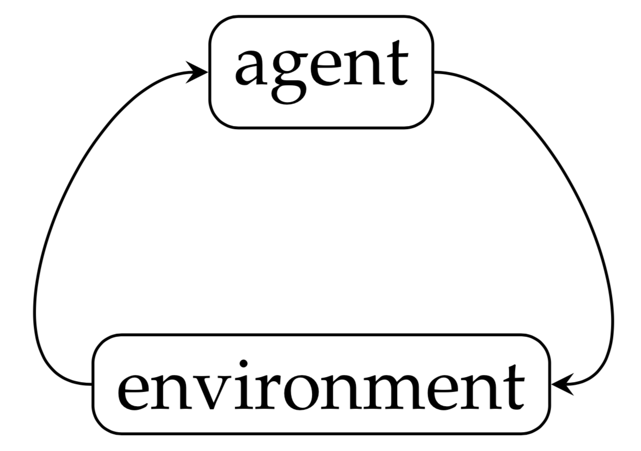
In step $t$, the agent takes an action and the action $a^{(t)}$ in turn would have an effect on the environment. As a result, the state of the environment goes from $s^{(t)}$ to $s^{(t+1)}$ and returns a reward $r^{(t+1)}$ to the agent. Usually, the goal in RL is to pick up actions so that the cumulative reward $\sum_{t=0}^{m}{r^{(t+1)}}$ is maximized. When ${m\to\infty}$, the cumulative reward may not bounded. In that case, the future reward can be discounted by $\lambda\in{[0, 1]}$ and we want to maximize $\sum_{t=0}^{\infty}{\lambda^{t}r^{(t+1)}}$. And in the following step, the agent would pick up the next action $a^{(t+1)}$ based on the information collected. In general, the environment state and reward at step $t$ are random variables. If the probability distribution of the next state and reward only depends on the current environment state and the action picked up, the Markov property holds which results in a Markov decision process (MDP). A majority of RL studies focus on Markov decision process MDP.

With the advance of deep learning, deep learning-based RL has made significant progress recently. Many DRL algorithms have been developed, such as deep Q-networks (DQN) algorithm which we would talk with more details in the next Section.

As we mentioned, usually there are no data to learn in RL. Both supervised and unsupervised learning need data to perform optimization on some objective functions. So does RL, in a different approach. RL can also be viewed as a simulation-based optimization approach, because RL runs simulations for the agent-environment interaction.

There are many RL algorithms available online. In the next section we would have a look at the DQN algorithm.

Deep Q-Networks

To introduce DQN we first define an action-value function $Q_{\pi}(s,a)$ and the optimal action-value function $Q_{\pi}^{*}(s,a)$. The action-value function is defined as

$$
\begin{equation}
Q_{\pi}(s,a)=E[R|s,a,\pi],
\label{eq:rl_e}
\end{equation}
$$
where $R$ denotes the random cumulative (discounted) rewards to obtain if the agents start from state $s$ and take the action $a$ and then always follow the policy(strategy) $\pi$.

Based on the definition of the action-value function, the optimal action-value function is defined as

$$
\begin{equation}
Q_{\pi}^{*}(s,a)=Q_{\pi}(s,a).
\label{eq:rl_e1}
\end{equation}
$$

The optimal action-value function represents the optimal expected cumulative (discounted) rewards to obtain if the agent start from state $s$, action $a$. If we know the exact optimal action-value function, it is easy to derive the optimal policy $\pi$ – we can just choose the action that maximizes $Q_{\pi}^{*}(s,a)$. But how to get the optimal action-value function is the key problem. And DQN aims at approximating the optimal action-value function by (deep) neural networks. Let $Q(s,a;\theta)$ denote the neural networks parameterized by $\theta$.

Compared with the vanilla DQN, double DQN is more commonly used due to its advantages. The training of these neural networks are still done in a supervised manner, i.e., specify a loss function and update the parameters based on gradient-based methods. An important idea to improve the performance of DQN is the experience replay which is a brilliant idea and worth learning, but we would not talk about it.

Let’s see how to do RL in practice. Although there are some RL tools in R, I recommend using Python because there are much matured tools in the deep learning eco-system. To find the optimal strategy of the game we talked in the previous Section, we will use two packages, i.e., gym ²⁹ and stable_baselines ³⁰. The gym package helps us define the environment and the stable_baselines package contains functionalities for building the DQN agent.

In gym there is a class Env based on which we can define our own environment class. More specifically, our environment class has to have three methods customized to fit the problem, i.e., the __init__ method, the reset method and the step method. The reset method specifies how to reset the environment before we start the learning. The step method specifies how the environment react to the action and it should return the next state and the reward. Also, step method should return if the current game is finished or not. Regarding our game, the state that the agent observes in each step could be the current time in the game, and the reward is always 1. If the current environment time is greater than the time horizon, the game is finished. We could define the environment class in the following code snippet.

Python

chapter7/game_env.py

 1 import numpy as np
 2 from gym import Env, spaces
 3 
 4 class GameEnv(Env):
 5     """
 6     H: the finite horizon of the game to specify
 7     """
 8     def __init__(self, H):
 9         self.H = H
10         # there are two actions available - 0 and 1, thus we use a discrete(2) space
11         self.action_space = spaces.Discrete(2)
12         # the observation/state has a single dimension to reflect the current environment time
13         self.observation_space = spaces.Box(low=np.array([0]), high=np.array([self.H]))
14         self.current_time = 0.0
15 
16     def reset(self):
17         self.current_time = 0.0
18         return np.array([self.current_time])
19 
20     def step(self, action):
21         if action == 0:
22             self.current_time += 1.0
23         elif action == 1:
24             self.current_time += 2.0
25         done = self.current_time >= self.H
26         reward = 1
27         info = {}
28         return np.array([self.current_time]), reward, done, info

And the code below shows how to use a DQN agent to play the game with the help of the stable_baselines package.

Python

chapter7/game_env_run.py

 1 import numpy as np
 2 from game_env_run import GameEnv
 3 from stable_baselines import DQN
 4 from stable_baselines.common.vec_env import DummyVecEnv
 5 from stable_baselines.deepq.policies import MlpPolicy
 6 
 7 if __name__ == "__main__":
 8     # the horizon of the game is 100 time units
 9     H = 100
10     # create the instance of our game environment
11     env = GameEnv(H)
12     env.reset()
13     # create the DQN agent with MlpPolicy which is a predefined neural network and our env instance
14     model = DQN(MlpPolicy, env, gamma=1.0, verbose=0)
15     # let's train the model with 20000 timesteps
16     model.learn(total_timesteps=20000)
17 
18     # now let's test our agent with 1000 games
19     n = 1000
20     env.reset()
21     r, a = [], []
22     for _ in range(n):
23         current_r = 0.0
24         obs = env.reset()
25         done = False
26         while not done:
27             action, _ = model.predict(obs)
28             obs, rewards, done, _ = env.step(action)
29             current_r += rewards
30             a.append(action)
31         r.append(current_r)
32     print("the average cumulative rewards from {0} games is {1}".format(
33         n, np.mean(r)))

By running the code above, we have the following output.

Python

1 chapter7 $python3.7 game_env_run.py
2 the average cumulative rewards from 1000 games is 100.0

In the game we discussed above, the environment does not have stochasticity and the optimal policy does not depend on the environment’s state at all as it is a simplified example to illustrate the usage of the tools. The real-world problems are usually much more complicated than the example, but we could follow the same procedure, i.e., define the environment for the problem and then build the agent for learning.

Computational differentiation

In Chapter 6 we talked about the gradient-based optimization algorithms, such as the vanilla gradient descent. We implemented the gradient descent method for linear regression. If you have used modern machine learning frameworks such as tensorflow, you may remember in tensorflow there is no need to define the gradient update step manually and instead the framework handled the update magically. That is because these frameworks have automatic differentiation implemented.

It is worth distinguishing numerical differentiation, symbolic differentiation and automatic differentiation. Symbolic differentiation ³¹ aims at finding the derivative of a given formula with respect to a specified variable. It takes a symbolic formula as input and also returns a symbolic formula. For example, by using symbolic differentiation we could simplify $\partial {(x^2+y^2)}/\partial{x}$ to $2x$. Numerical differentiation is often used when the expression/formula of the function is unknown (or in a black box, for example, a computer program). Compared with symbolic differentiation, numerical differentiation and automatic differentiation try to evaluate the derivative of a function at a fixed point. For example, we may want to know the value of $\partial{f(x,y)}/\partial{x}$ when $x=x_0;y=y_0$. The most basic formula for numerical differentiation is $\lim_{h \to 0} (f(x+h))-f(x))/h$. In implementation, this limit could be approximated by setting $h$ to a very small value, for example $1e-6$. Automatic differentiation also aims at finding the numerical values of derivatives, in a more efficient approach based on chain rule. However, unlike the numerical differentiation, automatic differentiation requires the exact function formula/structure. Also, Automatic differentiation does not need the approximation for the limit which is done in numerical differentiation. At the lowest level, it evaluate the derivatives based on symbolic rules. Thus automatic differentiation is partly symbolic and partly numerical ³⁵.

Let’s see an example how to do symbolic differentiation in R and Python.

1 > D(expression(x^2 + y^2), "x")
2 2 * x

Python

1 >>> import sympy
2 >>> x = sym.Symbol('x')
3 >>> y = sym.Symbol('y')
4 >>> f = x**2 + y**2
5 >>> sym.diff(f, x)
6 2*x

It’s worth noting there are many other symbolic operations we could do in R/Python, for example, symbolic integration.

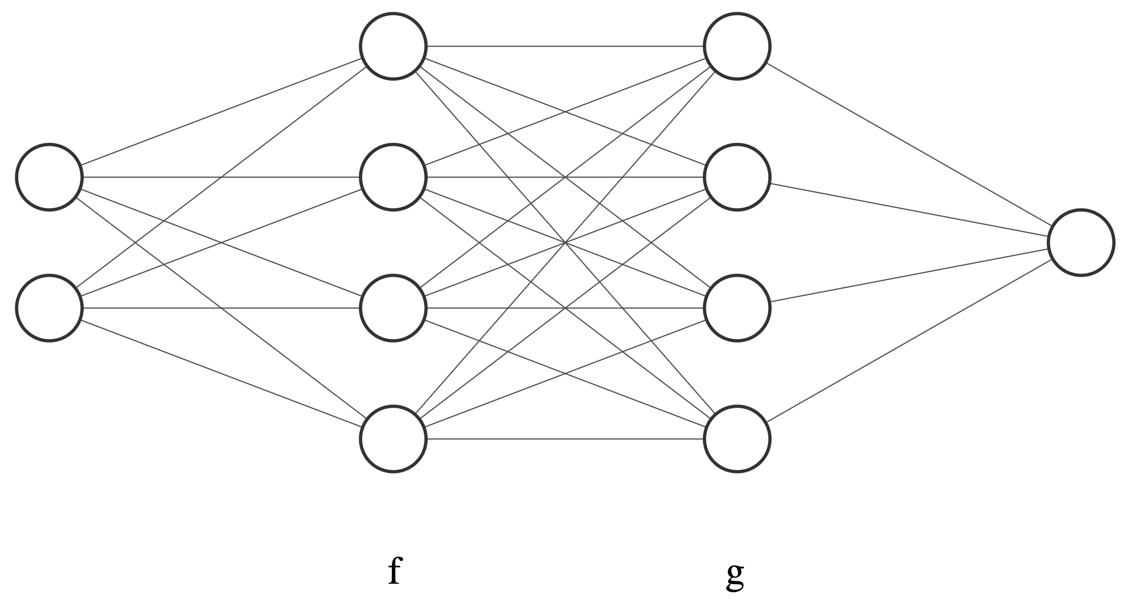
Automatic differentiation is extremely important in modern machine learning. Many deep learning models can be viewed as function compositions. Let’s take a two-hidden layer neural network illustrated below as an example. Let $x$ denote the input and $f_{u},g_{v}$ denote the first and second hidden layer, respectively. The output $y$ is written as $y=g_v(f_u(x))$. The learning task is to estimate the parameters $u,v$ in these hidden layers. If we use gradient descent approach for the parameter estimation, the evaluation of gradients for both $u$ and $v$ should be calculated. However, there might be overlapped operations if we simply perform two numerical differentiation operations independently. By utilizing automatic differentiation technique, it is possible to reduce the computational complexity.

A neural network with two hidden layers f and g

Let’s see how we could utilize the automatic differentiation to simply our linear regression implementation.

Python

chapter7/linear_regression_ad.py

 1 from autograd import grad
 2 import autograd.numpy as np
 3 
 4 class LR_AD:
 5     """
 6     linear regression using automatic differentiation from autograd
 7     """
 8     def __init__(self, x, y, learning_rate=0.005, seed=42):
 9         self.seed = seed
10         self.learning_rate = learning_rate
11         self.x = np.hstack((np.ones((x.shape[0], 1)), x))
12         self.y = y
13         self.coef = None
14 
15     def loss(self):
16         def loss_with_coef(coef):
17             y_hat = self.x @ coef
18             err = self.y - y_hat
19             return err @ err.T / self.x.shape[0]
20         # return the loss function with respect to the coef
21         return loss_with_coef
22 
23     def fit(self, max_iteration=1000):
24         # create the gradient function with the help of automatic differentiation
25         grad_func = grad(self.loss())
26         coef = np.random.uniform(size=(self.x.shape[1]))
27         for _ in range(max_iteration):
28             coef -= self.learning_rate*grad_func(coef)
29         self.coef = coef

In the implementation above, we use autograd.numpy to replace the ordinary numpy package in order to perform automatic differentiation on the functions of interest. In the loss method, we return a function loss_with_coef which captures the data required for the computation. This type of function is also called closure ³².

¹ Andrew R Barron. Universal approximation bounds for superpositions of a sigmoidal function. IEEE Transactions on Information theory, 39(3):930–945, 1993.

² https://docs.python.org/3/reference/import.html

³ https://en.wikipedia.org/wiki/Mean_absolute_error

⁴ https://en.wikipedia.org/wiki/Mean_absolute_percentage_error

⁵ https://en.wikipedia.org/wiki/Categorical_distribution

⁶ https://en.wikipedia.org/wiki/Precision_and_recall

⁷ https://en.wikipedia.org/wiki/Feature_engineering

⁸ https://en.wikipedia.org/wiki/Kolmogorov-Arnold_representation_theorem

⁹ Tomas Mikolov, Kai Chen, Greg Corrado, and Jeffrey Dean. Efficient estimation of word representations in vector space. arXiv preprint arXiv:1301.3781, 2013.

¹⁰ https://en.wikipedia.org/wiki/Autoencoder

¹¹ https://statisticalhorizons.com/multicollinearity

¹² https://github.com/r-lib/R6/issues/140

¹³ Tianqi Chen and Carlos Guestrin. Xgboost: A scalable tree boosting system. In Proceedings of the 22nd acm sigkdd international conference on knowledge discovery and data mining, pages 785–794. ACM, 2016.

¹⁴ https://en.wikipedia.org/wiki/Early_stopping

¹⁵ https://github.com/dmlc/xgboost

¹⁶ https://github.com/microsoft/LightGBM

¹⁷ https://github.com/catboost/catboost

¹⁸ https://scikit-learn.org/stable/modules/generated/sklearn.preprocessing.LabelEncoder.html

¹⁹ https://scikit-learn.org/stable/modules/generated/sklearn.preprocessing.OneHotEncoder.html

²⁰ https://en.wikipedia.org/wiki/Reinforcement_learning

²¹ https://en.wikipedia.org/wiki/Transfer_learning

²² https://en.wikipedia.org/wiki/Semi-supervised_learning

²³ https://en.wikipedia.org/wiki/Support-vector_machine

²⁴ https://en.wikipedia.org/wiki/Linear_discriminant_analysis

²⁵ https://en.wikipedia.org/wiki/Expectation-maximization_algorithm

²⁶ https://en.wikipedia.org/wiki/K-means_clustering

²⁷ https://deepmind.com/research/case-studies/alphago-the-story-so-far

²⁸ https://openai.com/projects/five

²⁹ https://gym.openai.com

³⁰ https://stable-baselines.readthedocs.io/en/master

³¹ https://www.cs.utexas.edu/users/novak/asg-symdif.html

³² https://en.wikipedia.org/wiki/Closure_(computer_programming)

³³ http://incompleteideas.net/book/the-book.html

³⁴ https://spinningup.openai.com/en/latest/

³⁵ https://arxiv.org/abs/1502.05767

Machine Learning - A gentle introduction

Supervised learning

Population & random sample

Universal approximation & overfitting

Universal approximation

Overfitting & cross-validation

Evaluation metrics

Feature engineering & embedding

Collinearity

Feature selection & parameter tuning

Gradient boosting machine

Decision tree

Tree growing in gradient boosting machine

Optimization of GBM

Unsupervised learning

Principal component analysis (PCA)

Mixture model

Clustering

Reinforcement learning

Deep Q-Networks

Computational differentiation