Sections in this Chapter:

• A refresher on distributions
• Inversion sampling & rejection sampling
• Joint distribution & copula
• Fit a distribution
• Confidence interval
• Hypothesis testing

We will see a few topics related to random variables (r.v.) and distributions in this chapter.

A refresher on distributions

Distributions describe the random phenomenon in terms of probabilities. Distributions are connected to random variables. A random variable is specified by its distribution. We know a r.v. could be either discrete or continuous. The number of calls received by a call center is an example of discrete r.v., and the amount of time taken to read this book is a continuous random variable.

There are infinite number of distributions. Many important distributions fall into some distribution families (i.e., a parametric set of probability distributions of a certain form). For example, the multivariate normal distribution belongs to exponential distribution family¹.

Cumulative distribution function (CDF) specifies how a real-valued random variable $X$ is distributed, i.e.,

$$
\begin{equation}\label{eq:4_0_1}
F_X(x)=P(X\le x).
\end{equation}
$$

It is worth noting that CDF is always monotonic.

When the derivative of CDF exists, we call the derivative of $F$ as the probability density function (PDF) which is denoted by the lower case $f_X$. PDF is associated with continuous random variables. For discrete random variables, the counterpart of PDF is called probability mass function (PMF). PMF gives the probability that a random variable equal to some value, but PDF does not represent probabilities directly.

The quantile function is the inverse of CDF, i.e.,

$$
\begin{equation}\label{eq:4_0_1_2}
Q_X(p)=inf \{ x\in \boldsymbol{R}:p\le F_X(x) \}.
\end{equation}
$$

PDF, CDF and Quantile functions are all heavily used in quantitative analysis. In R and Python, we can find a number of functions to evaluate these functions. The best known distribution should be univariate normal/Gaussian distribution. Let’s use Gaussian random variables for illustration.

 1 > # for reproducibility
 2 > set.seed(42) 
 3 > # draw samples
 4 > x = rnorm(10, mean=0, sd=2)
 5 > print(x)
 6  [1]  2.7419169 -1.1293963  0.7262568  1.2657252  0.8085366
 7  [6] -0.2122490  3.0230440 -0.1893181  4.0368474 -0.1254282
 8 > print(mean(x))
 9 [1] 1.094594
10 > print(sd(x))
11 [1] 1.670898
12 > # evaluate PDF
13 > d = dnorm(x, mean=0, sd=2)
14 > print(d)
15  [1] 0.07793741 0.17007297 0.18674395 0.16327110 0.18381928
16  [6] 0.19835103 0.06364496 0.19857948 0.02601446 0.19907926
17 > # evalute CDF
18 > p = pnorm(x, mean=0, sd=2)
19 > print(p)
20  [1] 0.9148060 0.2861395 0.6417455 0.7365883 0.6569923 0.4577418
21  [7] 0.9346722 0.4622928 0.9782264 0.4749971
22 > # evaluate quantile
23 > q = qnorm(p, mean=0, sd=2)
24 > print(q)
25  [1]  2.7419169 -1.1293963  0.7262568  1.2657252  0.8085366
26  [6] -0.2122490  3.0230440 -0.1893181  4.0368474 -0.1254282

We see that qnorm(pnorm(x))=x.

In Python, we use the functions in numpy and scipy.stats for the same purpose.

 1 >>> import scipy.stats
 2 >>> import numpy as np
 3 >>> import scipy.stats
 4 >>> np.random.seed(42)
 5 >>> x = np.random.normal(loc=0.0, scale=2.0, size=10)
 6 >>> print(x)
 7 [ 0.99342831 -0.2765286   1.29537708  3.04605971 -0.46830675 -0.46827391
 8   3.15842563  1.53486946 -0.93894877  1.08512009]
 9 >>> norm = scipy.stats.norm(loc=0.0, scale=2.0)
10 >>> d = norm.pdf(x)
11 >>> print(d)
12 [0.17632116 0.19757358 0.16172856 0.06254333 0.19407713 0.19407788
13  0.05732363 0.1485901  0.17865677 0.17217026]
14 >>> p = norm.cdf(x)
15 >>> print(p)
16 [0.69030468 0.44501577 0.74140679 0.93612438 0.40743296 0.40743933
17  0.94285637 0.77858846 0.31936529 0.70628362]
18 >>> q = norm.ppf(p) # ppf is the quantile function
19 >>> print(q)
20 [ 0.99342831 -0.2765286   1.29537708  3.04605971 -0.46830675 -0.46827391
21   3.15842563  1.53486946 -0.93894877  1.08512009]

A random variable could also be multivariate. In fact, the univariate normal distribution is a special case of multivariate normal distribution whose PDF is given in

$$
\begin{equation}\label{eq:4_0_1_3}
p(\boldsymbol{x};\boldsymbol{\mu},\boldsymbol{\Sigma})=\frac {1} {(2\pi)^{m/2}{|\boldsymbol{\Sigma|}}^{1/2}}\exp(-\frac 1 2 (\boldsymbol{x}-\boldsymbol{\mu})^T\boldsymbol{\Sigma}^{-1}(\boldsymbol{x}-\boldsymbol{\mu})),
\end{equation}
$$

where $\boldsymbol{\mu}$ is the mean and $\boldsymbol{\Sigma}$ is the covariance matrix of the random variable $\boldsymbol{x}$.

Sampling from distributions are involved in many algorithms, such as Monte Carlo simulation. First, let’s see a simple example in which we draw samples from a 3-dimensional normal distribution.

 1 > library(mvtnorm)
 2 > mu = c(1, 2)
 3 > cov = array(c(1.0, 0.5, 0.5, 2.0), c(2, 2))
 4 > set.seed(42)
 5 > x = rmvnorm(n = 1, mean = mu, sigma = cov)
 6 > print(x)
 7          [,1]     [,2]
 8 [1,] 2.221431 1.498778
 9 > d = dmvnorm(x, mean = mu, sigma = cov)
10 > print(d)
11 [1] 0.04007949
12 > p = pmvnorm(lower=-Inf, upper = x[1,], mean = mu, sigma = cov)
13 > print(p)
14 [1] 0.344201
15 attr(,"error")
16 [1] 1e-15
17 attr(,"msg")
18 [1] "Normal Completion"

 1 >>> from scipy.stats import multivariate_normal as mvn
 2 >>> mu = np.array([1,2])
 3 >>> cov = np.array([[1, 0.5],[0.5, 2]])
 4 >>> mvn.random_state.seed(42)
 5 >>> dist = mvn(mean = mu, cov = cov)
 6 >>> x = dist.rvs(size=1)
 7 >>> print(x)
 8 [1.16865045 2.72887797]
 9 >>> d = dist.pdf(x)
10 >>> print(d)
11 0.10533537790438291
12 >>> p = dist.cdf(x)
13 >>> print(p)
14 0.44523665187828293

Please note in the example above, we do not calculate the quantiles. For multivariable distributions, the quantiles are not necessary to be fixed points.

Inversion sampling & rejection sampling

Inversion sampling

Sampling from the Gaussian or other famous distributions could be as simple as just calling a function. What if we want to draw samples from any distribution with its CDF? Inversion sampling is a generic solution. The key idea of inversion sampling is that $F_{X}(x)$ is always following a uniform distribution between $0$ and $1$. There are two steps to draw a sample with inversion sampling approach.

• draw independent and identical (i.i.d.) distribution random variables $u_1,…,u_n$ which are uniformly distributed on from 0 to 1;
• calculate the quantiles $q_1,…,q_n$ for $u_1,…,u_n$ based on the CDF, and return $q_1,…,q_n$ as the desired samples to draw.

Let’s see how to use the inversion sampling technique to sample from exponential distribution with CDF $f_X(x;\lambda) = 1-e^{-\lambda x}$.

 1 > n=1000
 2 > set.seed(42)
 3 > # step 1, draw from uniform dist
 4 > u = runif(n=n, min=0,max=1)
 5 > # step 2, calculate the quantiles
 6 > lambda = 2.0
 7 > x = qexp(u, rate = lambda)
 8 > # the mean is close to 1/lambda
 9 > mean(x)
10 [1] 0.4818323

 1 >>> import numpy as np 
 2 >>> np.random.seed(42)
 3 >>> n=1000
 4 >>> # step 1, generate from uniform(0,1)
 5 ... u = np.random.uniform(low=0, high=1, size=n)
 6 >>> # step 2, calculate the quantile
 7 ... lamb = 2.0
 8 >>> q = -np.log(1-u)/lamb
 9 >>> np.mean(q)
10 0.4862529739826122

In the above R implementation, we used the builtin quantile function in step 2; however, for many distributions there are no builtin quantile functions available and thus we need to specify the quantile function by ourselves (illustrated in the Python implementation).

Rejection sampling

Rejection sampling is also a basic algorithm to draw samples for a random variable $X$ given its PDF $f_X$. The basic idea of rejection sampling is to draw samples for a random variable $Y$ with PDF $f_Y$ and accept the samples with probability $f_X(x)/(Mf_Y(x))$. $M$ is selected such that $f_X(x)/(Mf_Y(x))\le1$. If the sample generated is rejected, the sampling procedure is repeated until an acceptance. More theoretical details of rejection sampling can be found from the wikipedia ². The distribution $f_Y$ is called proposal distribution.

Let’s try to draw samples from an exponential distribution truncated between $0$ and $b$. The PDF of this random variable is specified by $f_X(x;\lambda, b) = \lambda e^{-\lambda x}/( 1-e^{-\lambda b})$.

A naive approach is to sample from the untruncated exponential distribution and only accept the samples smaller than $b$, which is implemented as follows.

 1 n=1000
 2 set.seed(42)
 3 lambda = 1.0
 4 b = 2.0
 5 x = rep(0, n)
 6 i = 0
 7 while (i<n){
 8   y = rexp(n = 1, rate = lambda)
 9   if (y>=b) {
10     i=i+1
11     x[i] = y
12   }
13 }

 1 import numpy as np 
 2 np.random.seed(42)
 3 lamb, b = 1.0, 2.0
 4 n=1000
 5 x = []
 6 i = 0
 7 while i<n:
 8   y = np.random.exponential(scale = lamb, size = 1)
 9   if y>=b:
10     x.append(y[0])
11     i+=1

After running the code snippets above, we have the samples stored in $x$ from the truncated exponential distribution.

Now let’s use the rejection sampling technique for this task. Since we want to sample the random variable between $0$ and $b$, one natural choice of the proposal distribution $f_Y$ is a uniform distribution between $0$ and $b$ and we choose $M=b\lambda/(1-e^{-\lambda b})$. As a result, the acceptance probability $f_X(x)/(Mf_Y(x))$ becomes $e^{-\lambda x}$.

 1 n=1000
 2 set.seed(42)
 3 lambda = 1.0
 4 b = 2.0
 5 x = rep(0, n)
 6 i = 0
 7 while (i<n){
 8   # sample from the proposal distribution
 9   y = runif(1, min = 0, max = b)
10   # calculate the acceptance probability
11   p = exp(-lambda*y)
12   if (runif(1)<=p) {
13     i=i+1
14     x[i] = y
15   }
16 }

 1 import numpy as np
 2 np.random.seed(42)
 3 lamb, b = 1.0, 2.0
 4 n = 1000
 5 x = []
 6 i = 0
 7 while i < n:
 8     # sample from the proposal distribution
 9     y = np.random.uniform(low=0, high=b)
10     # calculate the acceptance probability
11     p = np.exp(-lamb*y)
12     if p >= np.random.uniform():
13         x.append(y)
14         i += 1

We have seen the basic examples on how to draw samples with inversion samples and truncated samples. Now let’s work on a more challenging problem.

Without loss of generality, let’s consider a unit sphere, i.e., the radius $r=1$. We want to draw i.i.d. points from a unit sphere. The problem appears simple at a first glance – we could utilize the spherical coordinates system and draw samples for $\phi$ and $\theta$. Now the question is how to sample for $\phi$ and $\theta$. A straightforward idea is to draw independent and uniform samples $\phi$ from $0$ to $2\pi$ and $\theta$ from $0$ to $\pi$, respectively. However, this idea is incorrect which will be analyzed below.

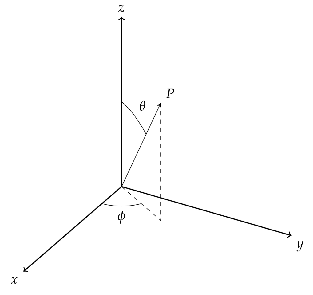
Let’s use $f_P(\phi,\theta)$ to denote the PDF of the joint distribution of $(\phi,\theta)$. We integrate this PDF, then

$$
\begin{equation}\label{eq:4_0_2}
1 = \int_{0}^{2\pi} \int_{0}^{\pi} f_P(\phi,\theta) d\phi d\theta = \int_{0}^{2\pi} \int_{0}^{\pi} f_\Phi(\phi) f_{\Theta|\Phi}(\theta|\phi) d\phi d\theta.
\end{equation}
$$

If we enforce $\Phi$ has a uniform distribution between $0$ and $2\pi$, then $f_\Phi(\phi)=1/{2\pi}$, and

$$
\begin{equation}\label{eq:4_0_3}
1=\int_{0}^{\pi} f_{\Theta|\Phi}(\theta|\phi) d\theta.
\end{equation}
$$

One solution to \eqref{eq:4_0_3} is $f_{\Theta|\Phi}(\theta|\phi)=sin(\theta)/2$.

Thus, we could generate the samples of $\Phi$ from the uniform distribution and the samples of $\Theta$ from the distribution whose PDF is $sin(\phi)/2$. Sampling for $\Phi$ is trivial, but how about $\Theta$? We could use the inversion sampling technique. The CDF of $\Theta$ is $(1-cos(\theta))/2;0\le\theta\le \pi$, and the quantile function is $Q_\Theta(p)=arccos(1-2p)$.

The implementation of sampling from unit sphere is implemented below.

 1 n=2000
 2 set.seed(42)
 3 # sample phi
 4 phi = runif(n, min = 0, max = 2*pi)
 5 # sample theta by inversion cdf
 6 u = runif(n, min = 0, max = 1)
 7 theta = acos(1-2*u)
 8 # now we calculate the Cartesian coordinates
 9 x = sin(theta)*cos(phi)
10 y = sin(theta)*sin(phi)
11 z = cos(theta)

 1 import numpy as np
 2 np.random.seed(42)
 3 n = 2000
 4 # sample phi
 5 phi = np.random.uniform(low=0, high=2*np.pi, size=n)
 6 # sample theta by inversion cdf
 7 u = np.random.uniform(low=0, high=1, size=n)
 8 theta = np.arccos(1-2*u)
 9 # we calculate the Cartesian coordinates
10 x = np.sin(theta)*np.cos(phi)
11 y = np.sin(theta)*np.sin(phi)
12 z = np.cos(theta)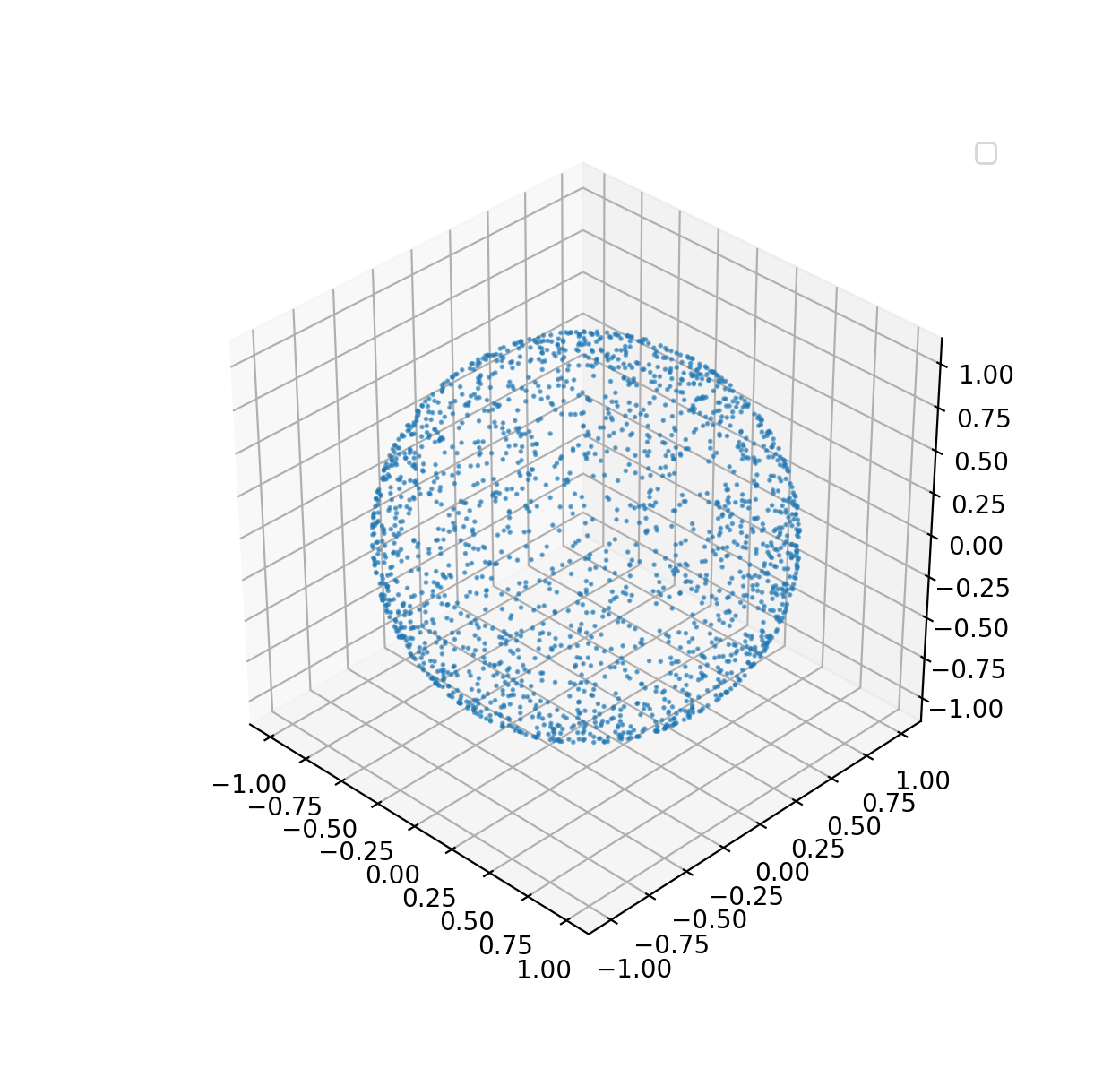

There are also other solutions to this problem, which wouldn’t be discussed in this book. A related problem is to draw samples inside a sphere. We could solve the inside sphere sampling problem with a similar approach, or using rejection sampling approach, i.e., sampling from a cube with acceptance ratio $\pi/6$.

Joint distribution & copula

We are not trying to introduce these concepts from scratch. This section is more like a recap.

In previous section, we see the PDF for multivariate normal distribution in \eqref{eq:4_0_1_3}. A multivariate distribution is also called joint distribution, since the multivariate random variable can be viewed as a joint of multiple univariate random variables. Joint PDF gives the probability density of a set of random variables. Sometimes we may only be interested in the probability distribution of a single random variable from a set. And that distribution is called marginal distribution. The PDF of a marginal distribution can be obtained by integrating the joint PDF over all the other random variables. For example, the integral of \eqref{eq:4_0_1_3} gives the PDF of a univariate normal distribution.

The joint distribution is the distribution about the whole population. In the context of a bivariate Gaussian random variable $(X_1,X_2)$, the joint PDF $f_{X_1,X_2}(x_1,x_2)$ specifies the probability density for all pairs of $(X_1,X_2)$ in the 2-dimension plane. The marginal distribution of $X_1$ is still about the whole population because we are not ruling out any points from the support of the distribution function. Sometimes we are interested in a subpopulation only, for example, the subset of $(X_1,X_2)$ where $X_2=2$ or $X_2>5$. We can use conditional distribution to describe the probability distribution of a subpopulation. To denote conditional distribution, the symbol $|$ is frequently used. We use $f_{X_1|X_2=0}(x_1|x_2)$ to represent the distribution of $X_1$ conditional on $X_2=0$. By the rule of conditional probability $P(A|B)=P(A,B)/P(B)$, the calculation $f_{X_1|X_2}(x_1|x_2)$ is straightforward, i.e., $f_{X_1|X_2}(x_1|x_2)=f_{X_1,X_2}(x_1,x_2)/f_{X_2}(x_2)$.

The most well-known joint distribution is the multivariate Gaussian distribution. Multivariate Gaussian distribution has many important and useful properties. For example, given the observation of $(X_1,…,X_k)$ from $(X_1,…,X_m)$, $(X_k+1,…,X_m)$ is still following a multivariate Gaussian distribution, which is essential to Gaussian process regression³.

We have seen the extension from univariate Gaussian distribution to multivariate Gaussian distribution, but how about other distributions? For example, what is the joint distribution for two univariate exponential distribution? We could use copula⁴ for such purpose. For the random variable $(X_1,…,X_m)$, let $(U_1,…,U_m)=(F_{X_1}(X_1),…,F_{X_m}(X_m))$ where $F_{X_k}$ is the CDF of $X_k$. We know $U_k$ is following a uniform distribution. Let $C(U_1,…,U_m)$ denote the joint CDF of $(U_1,…,U_m)$ and the CDF is called copula.

There are different copula functions, and one commonly-used is the Gaussian copula. The standard Gaussian copula is specified as below.

$$
\begin{equation}\label{eq:4_0_3_0}
C^{Gauss}_{\Sigma}(u_1,…,u_m)=\Phi_{\Sigma}(\Phi^{-1}(u_1),…,\Phi^{-1}(u_m)),
\end{equation}
$$

where $\Phi$ denotes the CDF of the standard Gaussian distribution, and $\Phi_{\Sigma}$ denotes the CDF of a multivariate Gaussian distribution with mean $\boldsymbol{0}$ and correlation matrix $\Sigma$.

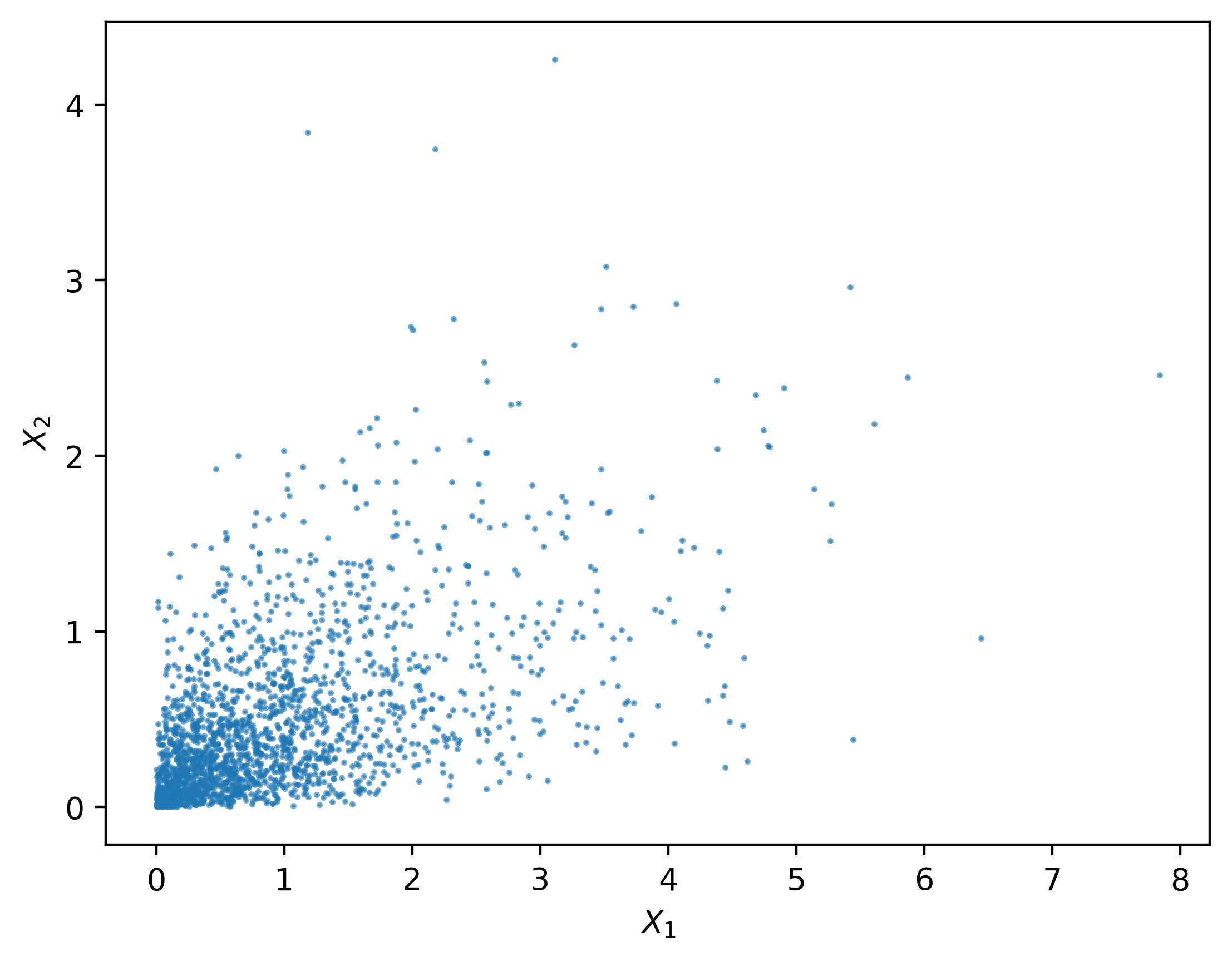
Let’s see an example to draw samples from a bivariate exponential distribution constructed via Gaussian copula. The basic idea of sampling multivariate random variables via copula is to sample $U_1,…,U_m$ first and then transform it to the desired random variables.

 1 > library(mvtnorm)
 2 > n = 10000
 3 > set.seed(42)
 4 > rates = c(1.0, 2.0)
 5 > mu = c(0, 0)
 6 > rho = 0.6
 7 > correlation = array(c(1, rho, rho, 1), c(2, 2))
 8 > # sample R from multivariate Gaussian
 9 > r = rmvnorm(n = n, mean = mu, sigma = correlation)
10 > # generate U
11 > u = pnorm(r)
12 > # calculate the quantile for X
13 > x1 = qexp(u[, 1], rate = rates[1])
14 > x2 = qexp(u[, 2], rate = rates[2])
15 > x = cbind(x1, x2)
16 > cor(x)
17           x1        x2
18 x1 1.0000000 0.5476137
19 x2 0.5476137 1.0000000
20 > apply(x, mean, MARGIN = 2)
21        x1        x2 
22 0.9934398 0.4990758

 1 >>> import numpy as np 
 2 >>> from scipy.stats import multivariate_normal as mvn
 3 >>> from scipy.stats import norm
 4 >>> mu = np.array([0, 0])
 5 >>> rho = 0.6
 6 >>> cov = np.array([[1, rho],[rho, 1]])
 7 >>> mvn.random_state.seed(42)
 8 >>> n = 10000
 9 >>> uvn = norm(loc=0.0, scale=1.0)
10 >>> dist = mvn(mean = mu, cov = cov)
11 >>> rates = [1.0, 2.0]
12 >>> # sample R from multivariate Gaussian
13 ... r = dist.rvs(size=n)
14 >>> # generate U
15 ... u = uvn.cdf(r)
16 >>> # calculate the quantile for X
17 ... def qexp(u, rate): return -np.log(1-u)/rate
18 ... 
19 >>> x1 = qexp(u[:, 0], rate = rates[0])
20 >>> x2 = qexp(u[:, 1], rate = rates[1])
21 >>> x = np.column_stack((x1, x2))
22 >>> np.corrcoef(x.T)
23 array([[1.        , 0.57359023],
24        [0.57359023, 1.        ]])
25 >>> np.mean(x, axis=0)
26 array([0.99768825, 0.50319692])

We plot 2000 samples generated from the bivariate exponential distribution constructed via copula in the figure below.

With the help of copula, we can even construct joint distribution with marginals from different distributions. For example, let’s make a joint distribution of a uniform distributed random variable and an exponential distributed random variable.

 1 > library(mvtnorm)
 2 > n = 10000
 3 > set.seed(42)
 4 > mu = c(0, 0)
 5 > rho = 0.6
 6 > correlation = array(c(1, rho, rho, 1), c(2, 2))
 7 > # sample R from multivariate Gaussian
 8 > r = rmvnorm(n = n, mean = mu, sigma = correlation)
 9 > # generate U
10 > u = pnorm(r)
11 > # calculate the quantile for X
12 > # X1 ~ exp(1.0); X2 ~ unif(0, 2)
13 > x1 = qexp(u[, 1], rate = 1.0)
14 > x2 = qunif(u[, 2], min = 0, max = 2)
15 > cor(x1, x2)
16 [1] 0.5220363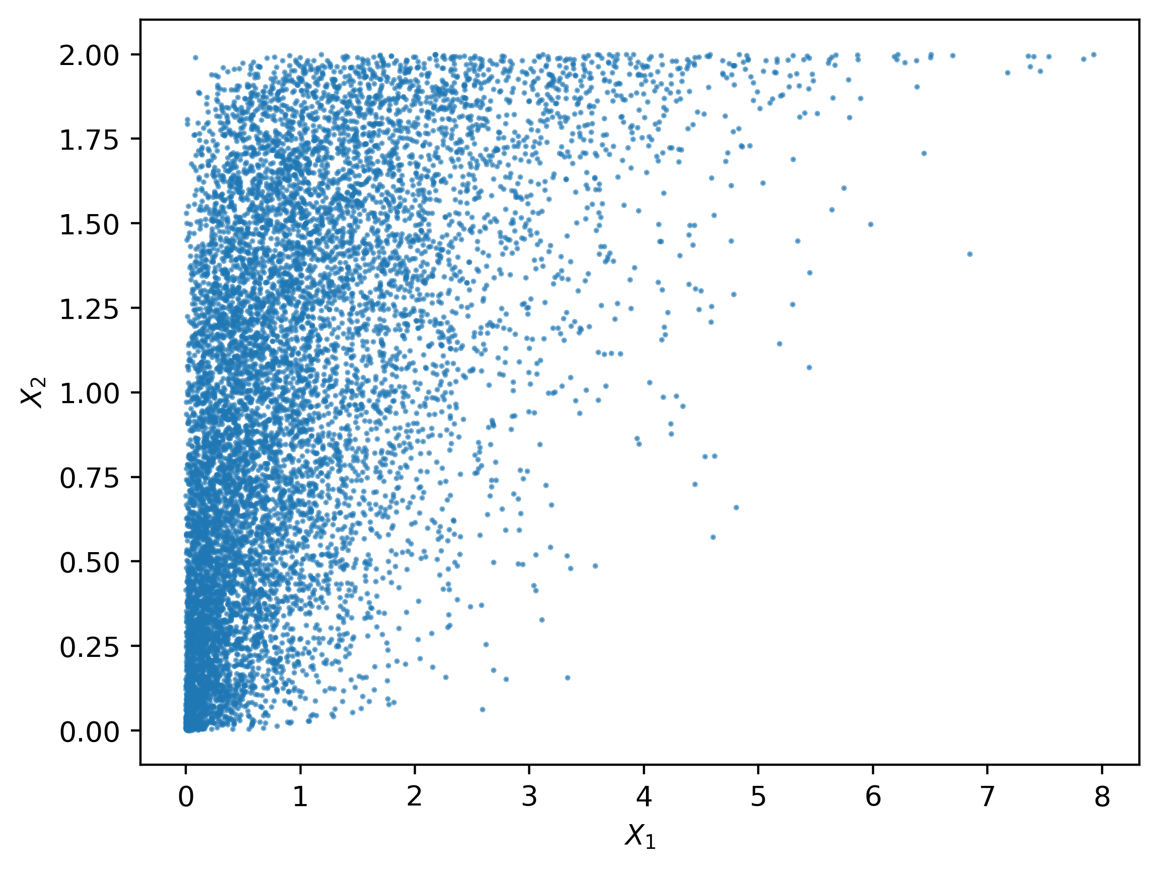

Fit a distribution

Statistics is used to solved real-world problems with data. In many cases we may have a collection of observations for a random variable and want to know the distribution which the observations follow. In fact, there are two questions involved in the process of fitting a distribution. First, which distribution to fit? And second, given the distribution how to estimate the parameters. These two questions are essentially the same questions that we have to answer in supervised learning. In supervised learning, we need to choose a model and estimate the parameters (if the model has parameters). We can also call these two questions as model selection and model fitting. Usually, model selection is done based on the model fitting.

Two widely-used methods in distribution fitting – method of moments and maximum likelihood method. In this Section we will see the method of moments. The maximum likelihood method would be introduced in Chapter 6. The $k^{th}$ moment of a random variable is defined as $\mu_k=E(x^k)$. If there are $m$ parameters, usually we derive the first $m$ theoretical moments in terms of the parameters, and by equating these theoretical moments to the sample moments $\hat{\mu_k}=1/n\sum_1^n{x_i^k}$ we will get the estimate.

Let’s take the univariate Gaussian distribution as an example. We want to estimate the mean $\mu$ and variance $\sigma^2$. The first and second theoretical moments is $\mu$ and $\mu^2+\sigma^2$. Thus, the estimate $\hat\mu$ and $\hat{\sigma}^2$ are $1/n\sum_1^n{x_i}$ and $1/n\sum_1^n{x_i^2}-(1/n\sum_1^n{x_i})^2=1/n\sum_1^n{(x_i-\hat\mu)^2}$. The code snippets below show the implementation.

 1 > set.seed(42)
 2 > n = 1000
 3 > mu = 2.5
 4 > var = 1.6
 5 > x = rnorm(n, mu, sqrt(var))
 6 > mu_est = mean(x)
 7 > var_est = mean((x-mu_est)^2)
 8 > print(mu_est)
 9 [1] 2.467334
10 > print(var_est)
11 [1] 1.60647

 1 >>> import numpy as np
 2 >>> np.random.seed(42)
 3 >>> n = 1000
 4 >>> mu, var = 2.5, 1.6
 5 >>> x = np.random.normal(2.5, 1.6**0.5, size=n)
 6 >>> mu_est = np.mean(x)
 7 >>> var_est = np.mean((x-mu_est)**2)
 8 >>> print(mu_est)
 9 2.524453331300827
10 >>> print(var_est)
11 1.5326479835704276

We could also fit another distribution to the data generated from a normal distribution. But which one is better? One answer is to compare the likelihood functions evaluated at the fitted parameters and choose the one that gives the larger likelihood value.

Please note that different methods to fit a distribution may lead to different parameter estimates. For example, the estimate of population variance using maximum likelihood method is different from that using moments method. Actually, the estimator for population mean is biased using methods method but the estimator using maximum likelihood method is unbiased.

Confidence interval

In the previous Section we have seen the parameter estimation of a distribution. However, the parameter estimates from either the method of moments or the maximum likelihood estimation are not the exact values of the unknown parameters. There are uncertainties associated with distribution fitting because the data to which the distribution is fit usually is just a random sample rather than a population. Suppose we could repeat the distribution fitting process $m$ times and each time we collect a random sample of size $n$ (i.e., a collection of $n$ observations for the random variable of interest), then we will get $n$ estimates of the distribution parameters. Which estimate is the best to use? In fact, all these $n$ estimates are observations of the estimator random variable. Estimator is a function of the random sample, and itself is a random variable. For example, eq1 is an estimator for the $\mu$ parameter in a Gaussian distribution.

Central limit theorem

Now we know when we fit a distribution, the parameter estimates are not the exact values of the unknown parameters. The question is how to quantify the uncertainties? To answer this question, we better know the distribution of the estimator. In the example of the Gaussian distribution, what distribution does the estimator $\hat\mu$ follow? It is straightforward to see that estimator is still following a Gaussian distribution since each $X_i$ is following a Gaussian distribution (sum of independent Gaussian random variables still follow a Gaussian distribution). But what if $X_i$ is from an arbitrary distribution? We may still derive an exact distribution of the sample mean $\hat{\mu}$ for an arbitrary distribution, but sometimes the derivation may not be easy. A simple idea is to use the central limit theorem (CLT), which states that the distribution of the mean of a random sample from a population with finite variance is approximately normally distributed when the sample size is large enough. More specifically, $\sqrt{n}(\bar{X}-\mu)/\sigma\xrightarrow{d} N(0,1)$ where $\mu$ and $\sigma$ are the population mean and standard deviation, respectively. Sometimes we do not have the actual value of the population standard deviation and the sample standard deviation $S$ can be used instead and thus $\sqrt{n}(\bar{X}-\mu)/S\xrightarrow{d} N(0,1)$.

We know if $Z$ is a Gaussian random variable, $P(- Z_{(1+\alpha)/2} < Z\le Z_{(1+\alpha)/2}) = \alpha$ where $Z_{u}$ denotes the quantile of $u$.
By CLT, $P(- Z_{(1+\alpha)/2} \le \sqrt{n}(\bar{X}-\mu)/S \le Z_{(1+\alpha)/2}) = \alpha$, which further leads to $P(\bar{X}- Z_{(1+\alpha)/2}S/\sqrt{n} \le \mu \le \bar{X}+ Z_{(1+\alpha)/2}S/\sqrt{n}) = \alpha$. The interval $\bar{X} \pm Z_{(1+\alpha)/2}S/\sqrt{n}$ is called an $\alpha$ confidence interval (CI) for the population mean $\mu$. For example, since $Z_{(1+0.95)/2}=1.96$ the 95% CI is constructed as $\bar{X} \pm 1.96S/\sqrt{n}$. Of course, if we know the exact value of $\sigma$, we could use $\bar{X} \pm 1.96\sigma/\sqrt{n}$ instead.

We show an example for the confidence interval calculation of population mean in normal distribution.
R

 1 > set.seed(42)
 2 > n = 1000
 3 > mu = 2.5
 4 > var = 1.6
 5 > x = rnorm(n, mu, sqrt(var))
 6 > mu_est = mean(x)
 7 > # we can also calculate S with sd(x) in R
 8 > S = sqrt(sum((x - mu_est) ^ 2) / (n - 1))
 9 > alpha = 0.95
10 > Z_alpha = qnorm((1 + alpha) / 2)
11 > CI = c(mu_est - Z_alpha * S / sqrt(n), mu_est + Z_alpha * S / sqrt(n))
12 > print(CI)
13 [1] 2.388738 2.545931

 1 >>> import numpy as np
 2 >>> import scipy
 3 >>> np.random.seed(42)
 4 >>> n = 1000
 5 >>> mu, var = 2.5, 1.6
 6 >>> norm = scipy.stats.norm(loc=0, scale=1)
 7 >>> x = np.random.normal(mu, var**0.5, size=n)
 8 >>> mu_est = np.mean(x)
 9 >>> S = np.sqrt(np.sum((x-mu_est)**2)/(n-1))
10 >>> alpha = 0.95
11 >>> Z_alpha = norm.ppf((1+alpha)/2)
12 >>> CI = [mu_est - Z_alpha*S/np.sqrt(n), mu_est + Z_alpha*S/np.sqrt(n)]
13 >>> print(CI)
14 [2.4476842124240363, 2.6012224501776178]

The interpretation of CI is tricky. A 95% CI does not mean the probability that the constructed CI contains the true population mean is $0.95$. Actually, a constructed CI again is a random variable because the CI is created based on each random sample collected. Following the classic explanation from textbooks, when we repeat the procedures to create CI multiple times, the probability that the true parameter falls into the CI is equal to $\alpha$. Let’s do an example to see that point.
R

 1 > set.seed(42)
 2 > B = 1000
 3 > n = 1000
 4 > mu = 2.5
 5 > var = 1.6
 6 > alpha = 0.95
 7 > Z_alpha = qnorm((1 + alpha) / 2)
 8 > coverage = rep(0, B)
 9 > for (i in 1:B) {
10 +   x = rnorm(n, mu, sqrt(var))
11 +   mu_est = mean(x)
12 +   S = sqrt(sum((x - mu_est) ^ 2) / (n - 1))
13 +   CI = c(mu_est - Z_alpha * S / sqrt(n), mu_est + Z_alpha * S / sqrt(n))
14 +   coverage[i] = (mu >= CI[1]) && (mu <= CI[2])
15 + }
16 > # the coverage probability should be close to alpha
17 > print(mean(coverage))
18 [1] 0.941

Bootstrap

So far we have seen how to create the CI for sample mean. What if we are interested in quantifying the uncertainty of other parameters, for example, the variance of a random variable? If we estimate these parameters with maximum likelihood method, we can still construct the CI in a similar approach with the large sample theory[]. However, we would not discuss it in this book.
Alternatively, we could use the bootstrap technique.

Bootstrap is simple yet powerful. It is a simulation-based technique. If we want to estimate a quantity $\theta$, first we write the estimator for $\theta$ as a function of a random sample i.e., $\hat{\theta}=g(X_1,…,X_n)$. Next, we just draw a random sample and calculate $\hat{\theta}$ and repeat this process $B$ times to get a collection of $\hat{\theta}$ denoted as $\hat{\theta}^{(1)},…,\hat{\theta}^{(B)}$. From these simulated $\hat{\theta}$, we could simply use the percentile $\hat{\theta}_{(1-\alpha)/2}$ and $\hat{\theta}_{(1+\alpha)/2}$ to construct the $\alpha$ CI. There are also other variants of bootstrapping method with similar ideas.

Let’s try to use bootstrap to construct a 95% CI for the population variance of a Gaussian distributed random variable.

 1 > set.seed(42)
 2 > B = 1000
 3 > n = 1000
 4 > mu = 2.5
 5 > var = 1.6
 6 > alpha = 0.95
 7 > Z_alpha = qnorm((1 + alpha) / 2)
 8 > var_sample = rep(0, B)
 9 > for (i in 1:B) {
10 +   x = rnorm(n, mu, sqrt(var))
11 +   var_sample[i] = sum((x-mean(x))^2)/(n-1)
12 + }
13 > quantile(var_sample, c((1-alpha)/2, (1+alpha)/2))
14     2.5%    97.5% 
15 1.466778 1.738675 

Hypothesis testing

We have talked about confidence interval, which is used to quantify the uncertainty in parameter estimation. The root cause of uncertainty in parameter estimation is that we do the inference based on random samples. Hypothesis testing is another technique related to confidence interval calculation.

A hypothesis test is an assertion about populations based on random samples. The assertion could be for a single population or multiple populations. When we collect a random sample, we may try to use the random sample as evidence to judge the hypothesis. Usually a hypothesis testing consists of two hypotheses:

• $H_0$: the null hypothesis;
• $H_1$: the alternative hypothesis.

When we perform a hypothesis testing, there are two possible outcomes, i.e., a) reject $H_0$ if the evidence is likely to support the alternative hypothesis, and b) do not reject $H_0$ because of insufficient evidence.

The key point to understand hypothesis testing is the significant level which is usually denoted as $\alpha$. When the null hypothesis is true, the rejection of null hypothesis is called type I error. And the significance level is the probability of committing a type I error. When the alternative hypothesis is true, the acceptance of null hypothesis is called type II error. And the probability of committing a type II error is denoted as $\beta$. $1-\beta$ is called the power of a test.

To conduct a hypothesis testing, there are a few steps to go. First we have to specify the null and alternative hypotheses, and the significance level. Next, we calculate the test statistic based on the data collected. Finally, we calculate the $p$-value. If the $p$-value is smaller than the significance level, we reject the null hypothesis; otherwise we accept it. Some books may describe a procedure to compare the test statistic with a critic region, which is essentially the same as the $p$-value approach. The real challenge to conduct a hypothesis testing is to calculate the $p$-value, whose calculation depends on which hypothesis test to use. Please note that the $p$-value itself is a random variable since it is calculated from the random sample. And when the null hypothesis is true, the distribution of $p$-value is uniform from $0$ to $1$.

$p$-value is also a conditional probability. A major misinterpretation about $p$-value is that it is the conditional probability that given the observed data the null hypothesis is true. Actually, $p$-value is the probability of the observation given the null hypothesis is true.

For many reasons, we will not go in-depth into the calculation of $p$-values in this book. But the basic idea is to figure out the statistical distribution of the test statistic. Let’s skip all the theories behind and go to the tools in R/Python.

One-sample $t$ test

Probably one-sample $t$ test is the most basic and useful hypothesis tests. It can determine if the sample mean is statistically different from a hypothesized population mean for continuous random variables. To use one-sample $t$ test some assumptions are usually required. For example, the observations should be independent. Another assumption is the normality, i.e., the population should be normal distributed or approximately normal distributed. However, the normality assumption is controversial but it is beyond the scope of this book.

In one-sample $t$ test, the alternative hypothesis could be two-sided, or one-sided. A two-sided $H_1$ does not specify if the population mean is greater or smaller than the hypothesized population mean. In contrast, a one-sided $H_1$ specifies the direction.

Now let’s see how to perform one-sample $t$ test in R/Python.

 1 > set.seed(42)
 2 > n = 50
 3 > mu = 2.5
 4 > sigma = 1.0
 5 > # set the significance level
 6 > alpha = 0.05
 7 > # sample 50 independent observations from a normal distribution
 8 > x = rnorm(n, mu, sigma)
 9 > mu_test = 2.5
10 > 
11 > # first, let's do two-sided t test
12 > # H0: the population mean is equal to mu_test
13 > # H1: the population mean is not equal to mu_test
14 > t1 = t.test(x, alternative = "two.sided", mu = mu_test)
15 > print(t1)
16 
17 	One Sample t-test
18 
19 data:  x
20 t = -0.21906, df = 49, p-value = 0.8275
21 alternative hypothesis: true mean is not equal to 2.5
22 95 percent confidence interval:
23  2.137082 2.791574
24 sample estimates:
25 mean of x 
26  2.464328 
27 
28 > # based on the p-value (> alpha), we accept the null hypothesis stated above
29 > t1$value
30 NULL
31 > 
32 > # next, let's do a one-sided t test
33 > # H0: the population mean is equal to mu_test
34 > # H1: the population mean is greater than mu_test
35 > t2 = t.test(x, alternative = "greater", mu = mu_test)
36 > print(t2)
37 
38 	One Sample t-test
39 
40 data:  x
41 t = -0.21906, df = 49, p-value = 0.5862
42 alternative hypothesis: true mean is greater than 2.5
43 95 percent confidence interval:
44  2.191313      Inf
45 sample estimates:
46 mean of x 
47  2.464328 
48 
49 > # based on the p-value (> alpha), we accept the null hypothesis stated above
50 > t2$p.value
51 [1] 0.5862418
52 > 
53 > # let's change mu_test and perform a one-sided test again
54 > mu_tes_new = 2.0
55 > t3 = t.test(x, alternative = "greater", mu = mu_tes_new)
56 > print(t3)
57 
58 	One Sample t-test
59 
60 data:  x
61 t = 2.8514, df = 49, p-value = 0.003177
62 alternative hypothesis: true mean is greater than 2
63 95 percent confidence interval:
64  2.191313      Inf
65 sample estimates:
66 mean of x 
67  2.464328 
68 
69 > # based on the p-value (< alpha), we reject the null hypothesis stated above, i.e., we conclude the population mean is greater than 2.
70 > t3$p.value
71 [1] 0.003177329

 1 >>> import numpy as np
 2 >>> from scipy.stats import ttest_1samp
 3 >>> np.random.seed(42)
 4 >>> n = 50
 5 >>> mu, sigma = 2.5, 1.0
 6 >>> # generate 50 independent samples from a normal distribution
 7 ... x = np.random.normal(mu, sigma, size=n)
 8 >>> alpha = 0.05
 9 >>> mu_test = 2.5
10 >>> # H0: population mean equals mu_test
11 ... # H1: population mean does not equal to mu_test
12 ... # perform a two-sided t test
13 ... t1 = ttest_1samp(x, mu_test)
14 >>> # based on the p-value (> alpha), we accept the null hypothesis stated aboveprint(t1.pvalue)
15 ... print(t1.pvalue)
16 0.09403837414922567

In the R code snippet we show both one-sided and two-sided one-sample $t$ tests. However, we only show a two-sided test in the Python program. It is feasible to perform a one-sided test in an indirect manner with the same function, but I don’t think it’s worth discussing here. For hypothesis testing, it seems R is a better choice than Python.

Two-sample $t$ test

Two-sample $t$ test is a bit of more complex than one-sample $t$ test. There are two types of $t$ tests commonly used in practice, i.e., paired $t$ test and unpaired $t$ test. In paired $t$ test, the samples are paired together. For example, we may want to know if there is a significant difference of the human blood pressures in morning and in evening. Hypothesis testing may help. To do so, we may conduct an experiment and collect the blood pressures in morning and in evening from a number of participants, respectively. Let $X_i$ denote the morning blood pressure and $Y_i$ denote the even blood pressure of participant $i$. We should pair $X_i$ and $Y_i$ since the pair is measured from the same person. Then the paired $t$ test can be used to compare the population means. The null hypothesis usually states that the difference of two population means is equal to a hypothesized value. Just like the one-sample $t$ test, we could do one-sided or two-sided paired $t$ test.

Now let’s see how to do paired $t$ test in R/Python.

 1 > library(mvtnorm)
 2 > set.seed(42)
 3 > n = 50
 4 > # we sample from a bivariate normal distribution
 5 > mu = c(2.0, 1.0)
 6 > sigma = diag(c(1.0, 1.5))
 7 > # significance level
 8 > alpha = 0.95
 9 > # sample 50 independent observations from the normal distribution
10 > mu_diff = 1.2
11 > x = rmvnorm(n, mu, sigma)
12 > 
13 > # first, let's do a two-sided t test
14 > # H0: the population means' difference is equal to mu_diff
15 > # H1: the population means' difference is not equal to mu_diff
16 > t.test(x=x[,1], y=x[,2], mu=mu_diff, paired = TRUE, alternative = "two.sided")
17 
18 	Paired t-test
19 
20 data:  x[, 1] and x[, 2]
21 t = -0.86424, df = 49, p-value = 0.3917
22 alternative hypothesis: true difference in means is not equal to 1.2
23 95 percent confidence interval:
24  0.5417625 1.4623353
25 sample estimates:
26 mean of the differences 
27                1.002049 
28 
29 > # we can't reject H0 based on the fact p-value>alpha
30 > 
31 > # next, let's do an one-sided t test
32 > # H0: the population means' difference is equal to mu_diff
33 > # H1: the population means' difference is less than mu_diff
34 > t.test(x=x[,1], y=x[,2], mu=mu_diff, paired = TRUE, alternative = "less")
35 
36 	Paired t-test
37 
38 data:  x[, 1] and x[, 2]
39 t = -0.86424, df = 49, p-value = 0.1958
40 alternative hypothesis: true difference in means is less than 1.2
41 95 percent confidence interval:
42      -Inf 1.386057
43 sample estimates:
44 mean of the differences 
45                1.002049 
46 
47 > # we can't reject H0 based on the fact p-value>alpha

Paired $t$ test can also be done in Python, but we would not show the examples.

Unpaired $t$ test is also about two population means’ difference, but the samples are not paired. For example, we may want to study if the average blood pressure of men is higher than that of women. In the unpaired $t$ test, we also have to specify if we assume the two populations have equal variance or not.

 1 > set.seed(42)
 2 > n = 50
 3 > alpha = 0.05
 4 > mu1 = 2.0
 5 > mu2 = 1.0
 6 > sigma1 = 1.0
 7 > sigma2 = 1.5
 8 > # generate two samples independently
 9 > x1 = rnorm(n, mu1, sigma1)
10 > x2 = rnorm(n, mu2, sigma2)
11 > # first, let's do a two-sided t test
12 > # assume equal variance for the two populations
13 > mu_diff = 0.5
14 > # H0: the population means' difference is equal to mu_diff
15 > # H1: the population means' difference is not equal to mu_diff
16 > t.test(x1, x2, alternative = "two.sided", mu = mu_diff, paired = FALSE, var.equal = TRUE)
17 
18 	Two Sample t-test
19 
20 data:  x1 and x2
21 t = 1.2286, df = 98, p-value = 0.2222
22 alternative hypothesis: true difference in means is not equal to 0.5
23 95 percent confidence interval:
24  0.3072577 1.3192945
25 sample estimates:
26 mean of x mean of y 
27  1.964328  1.151052 
28 
29 > # we accept the null hypothesis since p-value>alpha 
30 > 
31 > # now, we don't assume the equal variance
32 > t.test(x1, x2, alternative = "two.sided", mu = mu_diff, paired = FALSE, var.equal = FALSE)
33 
34 	Welch Two Sample t-test
35 
36 data:  x1 and x2
37 t = 1.2286, df = 94.78, p-value = 0.2223
38 alternative hypothesis: true difference in means is not equal to 0.5
39 95 percent confidence interval:
40  0.3070428 1.3195094
41 sample estimates:
42 mean of x mean of y 
43  1.964328  1.151052 
44 
45 > # there is no big change for p-value, we also accept the null hypothesis since p-value>alpha 
46 > 
47 > # let's try a one sided test without equal variance
48 > # H0: the population means' difference is equal to mu_diff
49 > # H1: the population means' difference larger than mu_diff
50 > t.test(x1, x2, alternative = "less", mu = mu_diff, paired = FALSE, var.equal = FALSE)
51 
52 	Welch Two Sample t-test
53 
54 data:  x1 and x2
55 t = 1.2286, df = 94.78, p-value = 0.8889
56 alternative hypothesis: true difference in means is less than 0.5
57 95 percent confidence interval:
58      -Inf 1.236837
59 sample estimates:
60 mean of x mean of y 
61  1.964328  1.151052 
62 
63 > # we accept the null hypothesis since p-value>alpha

There are many other important hypothesis tests, such as the chi-squared test⁵, likelihood-ratio test⁶.

¹ https://en.wikipedia.org/wiki/Exponential_family

² https://en.wikipedia.org/wiki/Rejection_sampling

³ http://www.gaussianprocess.org/gpml/chapters/RW2.pdf

⁴ https://en.wikipedia.org/wiki/Copula_(probability_theory)

⁵ https://en.wikipedia.org/wiki/Chi-squared_test

⁶ https://en.wikipedia.org/wiki/Likelihood-ratio_test